AFRICAST

Tidy time series & forecasting in R

Cross-validation and residual diagnostics

Session 9 of 10

tsibble feasts fable
workshop.f4sg.org/africastForecasting for Social Good

Time series cross-validation

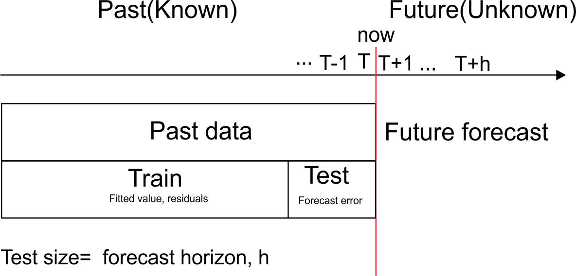
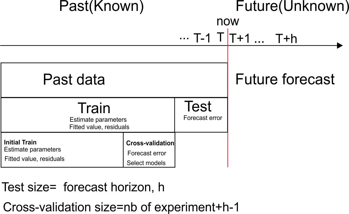
Issue with traditional train/test split

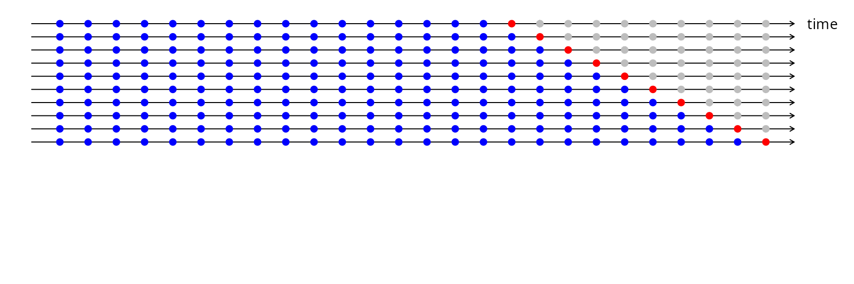
Forecasting from a rolling origin

Time series cross-validation

  • Forecast accuracy averaged over test sets.
  • Also known as “evaluation on a rolling forecasting origin”

Creating the rolling training sets

Three functions roll a tsibble into windows, numbered by a new .id column.

  • stretch_tsibble(): extends a growing window with new data.
  • slide_tsibble(): shifts a fixed length window through the data.
  • tile_tsibble(): moves a fixed length window without overlap.

For time series cross-validation, stretching windows are most commonly used.

Stretch: stretch_tsibble()

x <- tsibble(t = 1:20, index = t)
stretch <- x |> stretch_tsibble(.init = 6, .step = 2)

A tsibble x of 20 observations.

The first window holds the first .init = 6 observations.

The next window adds .step = 2 observations.

Keep growing until the window reaches the end of the data: 8 windows, numbered by .id.

Slide: slide_tsibble()

slide <- x |> slide_tsibble(.size = 8, .step = 2)

A tsibble x of 20 observations.

The first window holds the first .size = 8 observations.

The next window moves along by .step = 2 observations, keeping its size.

Keep sliding until the window reaches the end of the data: 7 windows.

Tile: tile_tsibble()

tile <- x |> tile_tsibble(.size = 5)

A tsibble x of 20 observations.

The first tile holds the first .size = 5 observations.

The next tile starts where the last ended, so the tiles never overlap.

Keep tiling until the data are used up: 4 tiles.

Rolling origins for drug sales

Monthly antidiabetic drug sales in Australia ($ millions), from 2000. Stretch with a minimum length of 24, growing by 1 each step.

forecast_horizon <- 12
test <- antidiabetic_drug_sale |> 
  slice((n()-forecast_horizon+1):n())
train <- antidiabetic_drug_sale |> 
  slice(1:(n()-forecast_horizon))
drug_sale_tcsv <- train |>
  stretch_tsibble(.init = 24, .step = 1)
# A tsibble: 3,819 x 3 [1M]
# Key:       .id [67]
     Month  Cost   .id
     <mth> <dbl> <int>
1 2000 Jan 12.5      1
2 2000 Feb  7.46     1
3 2000 Mar  8.59     1
4 2000 Apr  8.47     1
# ℹ 3,815 more rows

Fit models to each window

Estimate seasonal naïve, naïve and drift models for each window.

drug_fit_tr <- drug_sale_tcsv |> 
  model(
    snaive = SNAIVE(Cost),
    naive = NAIVE(Cost),
    drift = RW(Cost ~ drift())
  )
# A mable: 67 x 4
# Key:     .id [67]
    .id   snaive   naive         drift
  <int>  <model> <model>       <model>
1     1 <SNAIVE> <NAIVE> <RW w/ drift>
2     2 <SNAIVE> <NAIVE> <RW w/ drift>
3     3 <SNAIVE> <NAIVE> <RW w/ drift>
4     4 <SNAIVE> <NAIVE> <RW w/ drift>
# ℹ 63 more rows

Forecasts from each window

Produce 12-step-ahead forecasts from each model and window.

drug_fc_tr <- drug_fit_tr |> 
  forecast(h = forecast_horizon)
# A fable: 2,412 x 5 [1M]
# Key:     .id, .model [201]
    .id .model    Month        Cost .mean
  <int> <chr>     <mth>      <dist> <dbl>
1     1 snaive 2002 Jan  N(14, 1.7) 14.5 
2     1 snaive 2002 Feb   N(8, 1.7)  8.05
3     1 snaive 2002 Mar  N(10, 1.7) 10.3 
4     1 snaive 2002 Apr N(9.8, 1.7)  9.75
# ℹ 2,408 more rows

Which method will win?

Which method do you expect to forecast antidiabetic drug sales best?

  • Seasonal naïve
  • Naïve
  • Drift

Cross-validated accuracy

drug_fc_tr |>
  accuracy(
    antidiabetic_drug_sale,
    measures = list(
      point_accuracy_measures,
      interval_accuracy_measures,
      distribution_accuracy_measures
    )
  ) |>
  select(.model, RMSE, MAE, MASE, winkler, CRPS)
# A tibble: 3 × 6
  .model  RMSE   MAE  MASE winkler  CRPS
  <chr>  <dbl> <dbl> <dbl>   <dbl> <dbl>
1 drift   3.95  3.05  1.89    27.0  2.43
2 naive   3.87  2.96  1.84    25.0  2.31
3 snaive  2.42  1.94  1.20    15.3  1.42

Errors are averaged over all origins and all 12 horizons.

From cross-validation to forecasts

Seasonal naïve wins the cross-validation. How do you produce the forecasts you deliver?

  • Use the forecasts from the last window
  • Refit seasonal naïve on all the data
  • Average the forecasts from every window

Residual diagnostics

Forecasting residuals

Residuals in forecasting: difference between observed value and its fitted value (one-step forecast) on the training data: \(e_t = y_t-\hat{y}_{t|t-1}\).

Assumptions

  1. \(\{e_t\}\) uncorrelated. If they aren’t, then information left in residuals that should be used in computing forecasts.
  2. \(\{e_t\}\) have mean zero. If they don’t, then forecasts are biased.

Useful properties (for prediction intervals)

  1. \(\{e_t\}\) have constant variance.
  2. \(\{e_t\}\) are normally distributed.

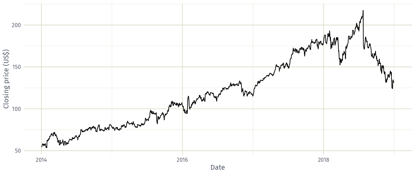
Facebook closing stock price

fb_stock <- gafa_stock |>
  filter(Symbol == "FB")
fb_stock |>
  autoplot(Close) +
  labs(x = "Date", y = "Closing price (US$)")
Naïve model of Facebook’s stock price

fb_stock <- fb_stock |>
  mutate(trading_day = row_number()) |>
  update_tsibble(index = trading_day, regular = TRUE)
fit <- fb_stock |> model(NAIVE(Close))
augment(fit)
# A tsibble: 1,258 x 7 [1]
# Key:       Symbol, .model [1]
   Symbol .model       trading_day Close .fitted .resid .innov
   <chr>  <chr>              <int> <dbl>   <dbl>  <dbl>  <dbl>
 1 FB     NAIVE(Close)           1  54.7    NA   NA     NA    
 2 FB     NAIVE(Close)           2  54.6    54.7 -0.150 -0.150
 3 FB     NAIVE(Close)           3  57.2    54.6  2.64   2.64 
 4 FB     NAIVE(Close)           4  57.9    57.2  0.720  0.720
 5 FB     NAIVE(Close)           5  58.2    57.9  0.310  0.310
 6 FB     NAIVE(Close)           6  57.2    58.2 -1.01  -1.01 
 7 FB     NAIVE(Close)           7  57.9    57.2  0.720  0.720
 8 FB     NAIVE(Close)           8  55.9    57.9 -2.03  -2.03 
 9 FB     NAIVE(Close)           9  57.7    55.9  1.83   1.83 
10 FB     NAIVE(Close)          10  57.6    57.7 -0.140 -0.140
# ℹ 1,248 more rows

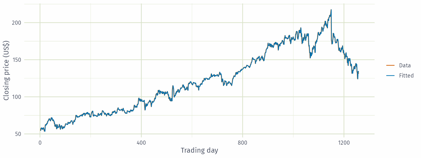
Fitted values

augment(fit) |>
  ggplot(aes(x = trading_day)) +
  geom_line(aes(y = Close, colour = "Data")) +
  geom_line(aes(y = .fitted, colour = "Fitted")) +
  labs(x = "Trading day", y = "Closing price (US$)", colour = NULL)
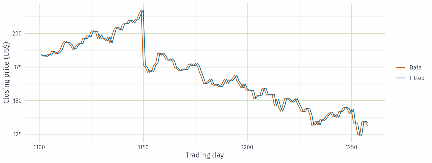
Fitted values (last 158 trading days)

augment(fit) |>
  filter(trading_day > 1100) |>
  ggplot(aes(x = trading_day)) +
  geom_line(aes(y = Close, colour = "Data")) +
  geom_line(aes(y = .fitted, colour = "Fitted")) +
  labs(x = "Trading day", y = "Closing price (US$)", colour = NULL)
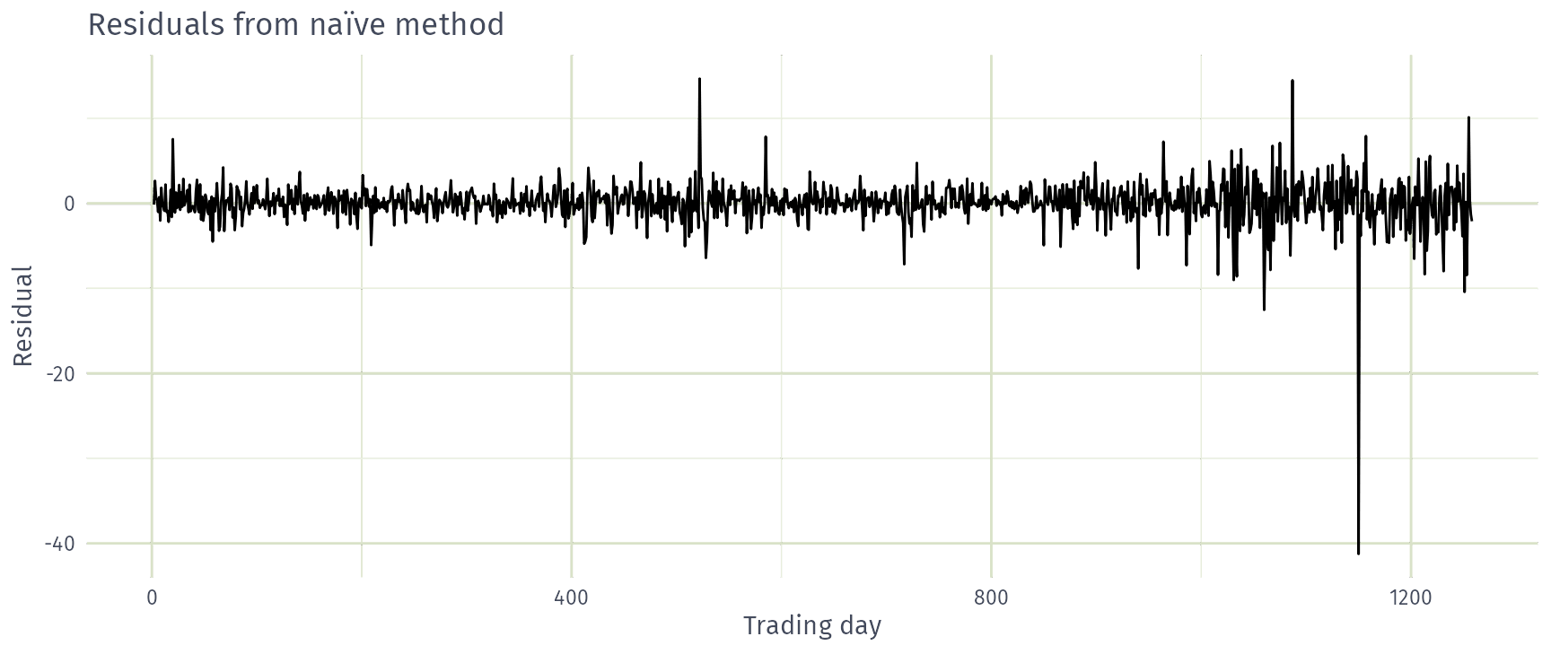
Residuals over time

augment(fit) |>
  autoplot(.resid) +
  labs(x = "Trading day", y = "Residual", title = "Residuals from naïve method")
Constant variance?
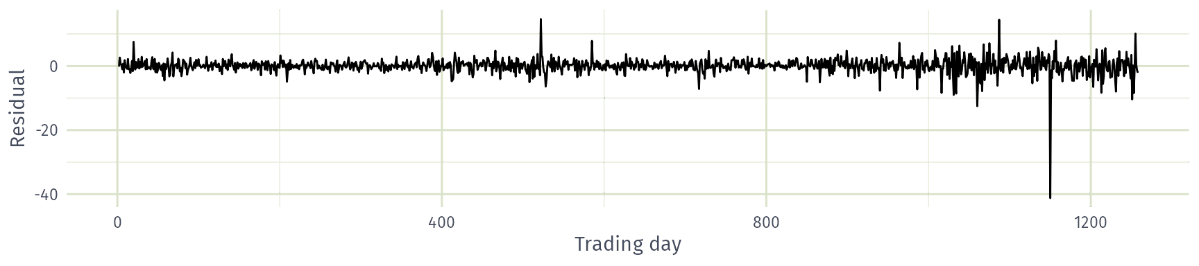
Do these residuals have constant variance?

  • Yes
  • No

Histogram of residuals

augment(fit) |>
  ggplot(aes(x = .resid)) +
  geom_histogram(bins = 150) +
  labs(x = "Residual", y = "Count", title = "Histogram of residuals")
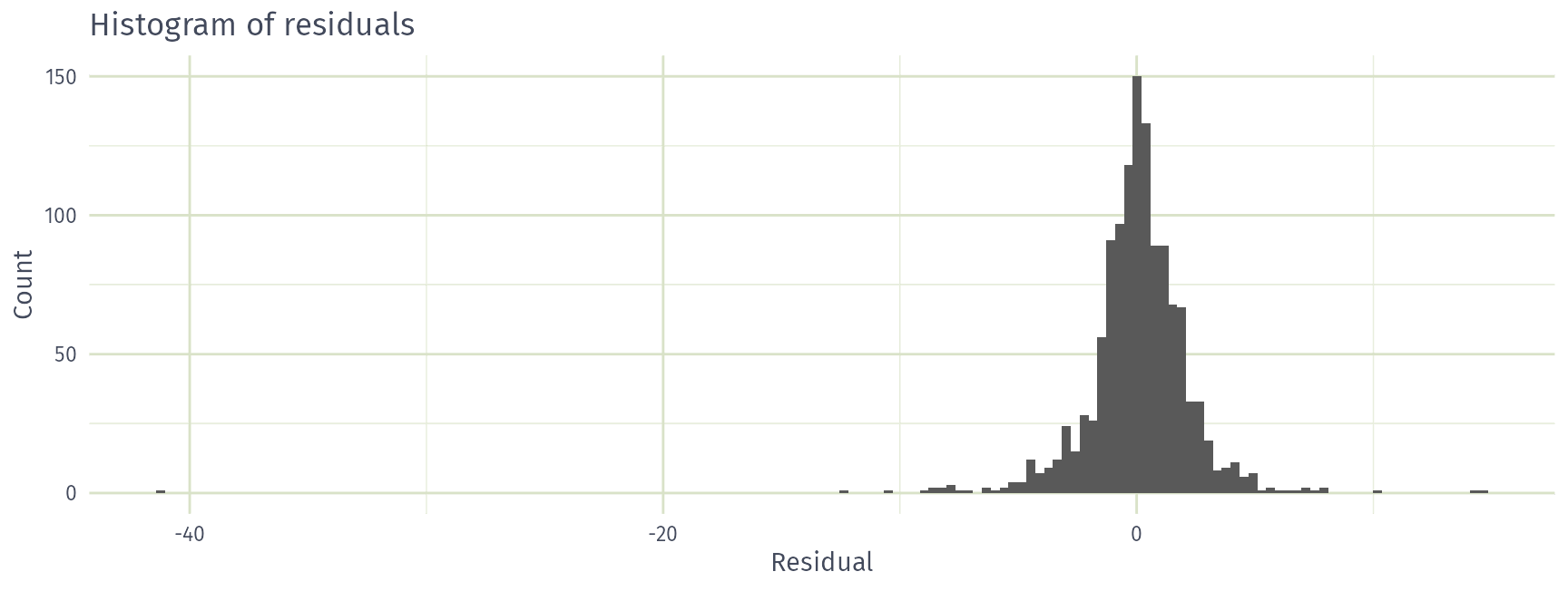
Normally distributed?
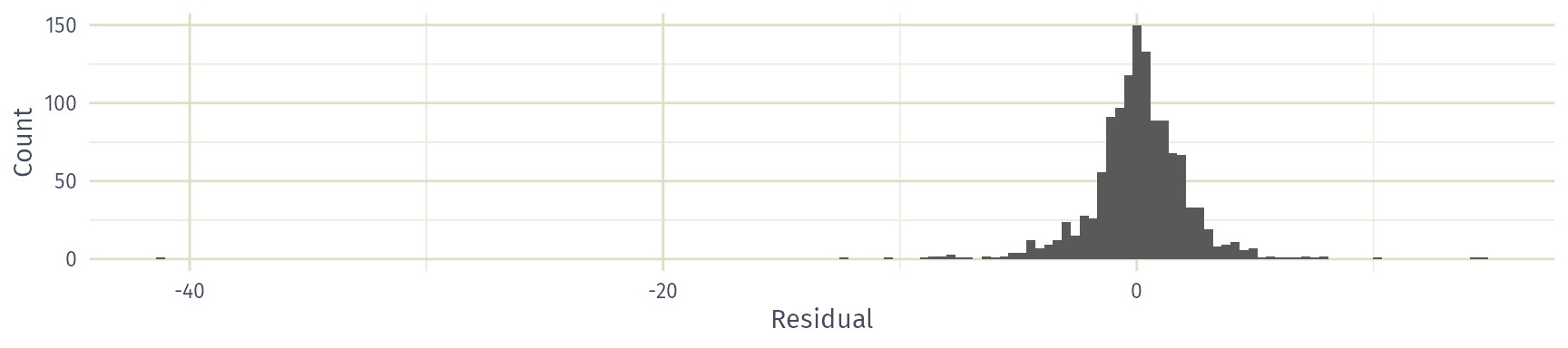
Do these residuals look normally distributed?

  • Yes
  • No

ACF of residuals

augment(fit) |>
  ACF(.resid) |>
  autoplot() +
  labs(x = "Lag", y = "ACF", title = "ACF of residuals")
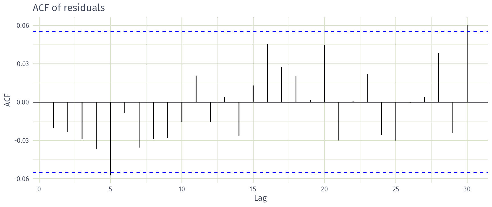
White noise?
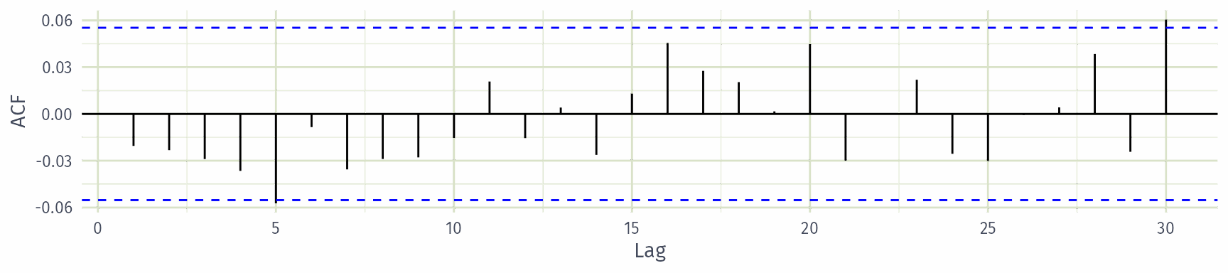
Do these residuals look like white noise?

  • Yes
  • No

Checking the ACF of residuals

  • We assume that the residuals are white noise (uncorrelated, mean zero, constant variance). If they aren’t, then there is information left in the residuals that should be used in computing forecasts.

  • So a standard residual diagnostic is to check the ACF of the residuals of a forecasting method.

  • We expect these to look like white noise.

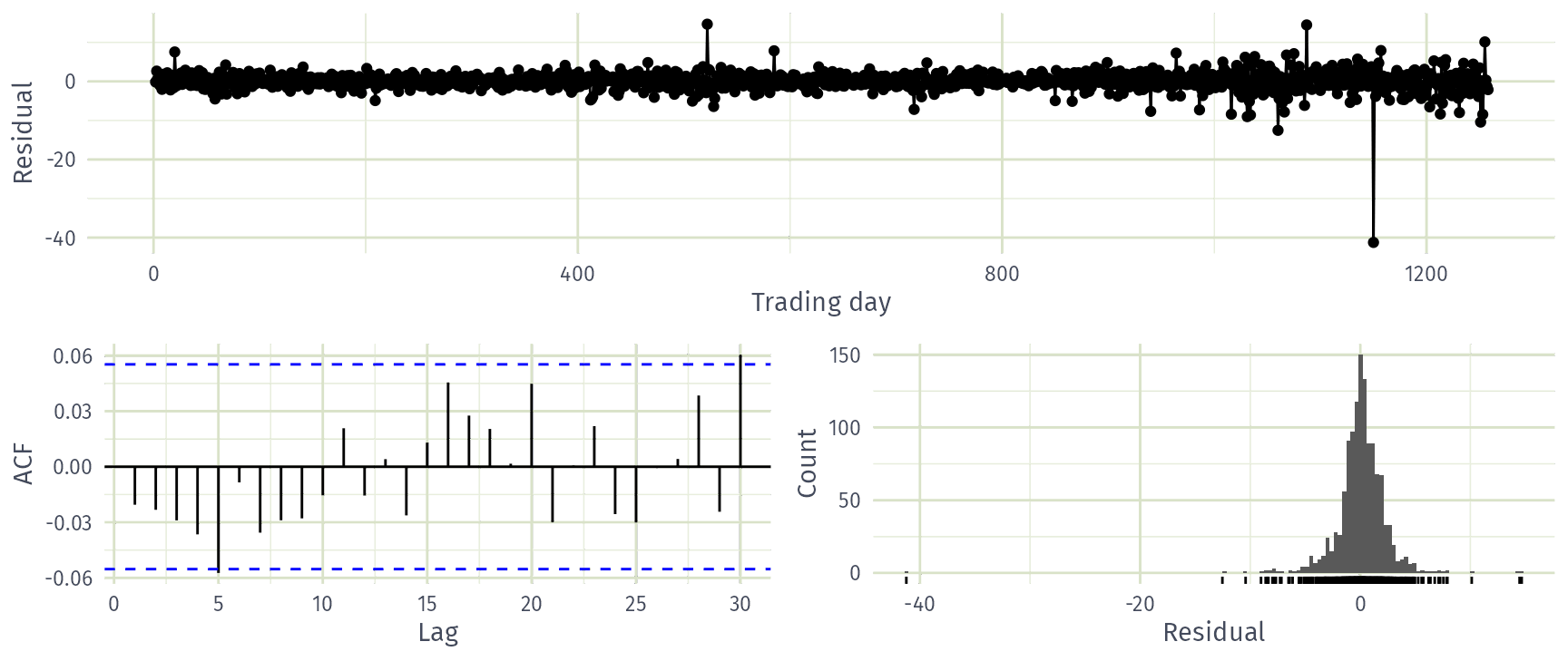
Combined diagnostic graph

fit |> gg_tsresiduals()
Ljung-Box test: recap

Recall from the regression session: test whether the first \(\ell\) autocorrelations \(r_k\) of the residuals are jointly zero.

\(\displaystyle Q = T(T+2) \sum_{k=1}^\ell (T-k)^{-1}r_k^2\)

  • Small \(Q\) (large \(p\)-value): consistent with white noise.
  • \(\ell=10\) for non-seasonal data, \(\ell=2m\) for seasonal data (at most \(T/5\)); dof \(= K\) estimated parameters.

Ljung-Box test of the naïve residuals

augment(fit) |> features(.resid, ljung_box, lag = 10)
# A tibble: 1 × 4
  Symbol .model       lb_stat lb_pvalue
  <chr>  <chr>          <dbl>     <dbl>
1 FB     NAIVE(Close)    12.1     0.276

\(p = 0.276 > 0.05\): no evidence against white noise.

What the residuals tell us

  • Mean close to zero: the forecasts are unbiased.
  • Uncorrelated: no information is left in the residuals.
  • Variance is not constant: it grows later in the series.
  • Heavy tails and a large outlier: the residuals are not normal.

The point forecasts are fine, but the prediction intervals may be inaccurate.

Recap

Recap

  • Time series cross-validation averages forecast accuracy over many rolling origins, not a single test set.
  • Roll the training data into windows with stretch_tsibble(), fit models to each window, forecast and compare with accuracy().
  • Residual diagnostics check that the best model’s residuals are uncorrelated with mean zero, and ideally have constant variance and are normal.
  • Check them with gg_tsresiduals() and the Ljung-Box test before forecasting.