AFRICAST

Tidy time series & forecasting in R

Exponential smoothing

Session 7 of 10

workshop.f4sg.org/africastForecasting for Social Good

Exponential smoothing

From simple methods to Exponential Smoothing

• Naive method: Use only the last observation.
• Average method: Use all observations.
• Want something in between naive and average methods.
• Most recent data should have more weight.
• This is exactly the concept behind exponential smoothing.

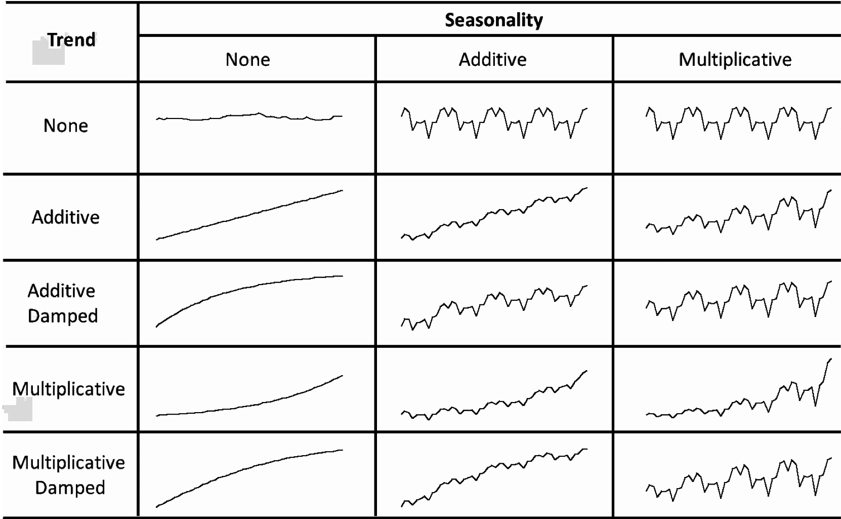
Pegels’ classification

Historical perspective

• Developed in the 1950s and 1960s as methods (algorithms) to produce point forecasts.
• Combine a “level”, “trend” (slope) and “seasonal” component to describe a time series.
• The rate of change of the components are controlled by “smoothing parameters”: \(\alpha\), \(\beta\) and \(\gamma\) respectively.
• Need to choose best values for the smoothing parameters (and initial states).
• Equivalent ETS state space models developed in the 1990s and 2000s.

A model for levels, trends, and seasonalities

We want a model that captures the level (\(\ell_t\)), trend (\(b_t\)) and seasonality (\(s_t\)).

How do we combine these elements?

Additively?

\(y_t = \ell_{t-1} + b_{t-1} + s_{t-m} + \varepsilon_t\)

Multiplicatively?

\(y_t = \ell_{t-1}b_{t-1}s_{t-m}(1 + \varepsilon_t)\)

Perhaps a mix of both?

\(y_t = (\ell_{t-1} + b_{t-1}) s_{t-m} + \varepsilon_t\)

How do the level, trend and seasonal components evolve over time?

ETS models

General notation    E T S :  ExponenTial Smoothing

\(\nearrow\)	\(\uparrow\)	\(\nwarrow\)
Error	Trend	Season

Error: Additive ("A") or multiplicative ("M")

Trend: None ("N"), additive ("A"), multiplicative ("M"), or damped ("Ad" or "Md").

Seasonality: None ("N"), additive ("A") or multiplicative ("M")

ETS(A,N,N): SES with additive errors

\[\begin{aligned} \text{Forecast equation}&& \hat{y}_{T+h|T} &= \ell_T \\ \text{Measurement equation}&& y_t &= \ell_{t-1} + \varepsilon_t\\ \text{State equation}&& \ell_t&=\ell_{t-1}+\alpha \varepsilon_t \end{aligned}\]

where \(\varepsilon_t\sim\text{NID}(0,\sigma^2)\).

• “innovations” or “single source of error” because equations have the same error process, \(\varepsilon_t\).
• Measurement equation: relationship between observations and states.
• Transition/state equation(s): evolution of state(s) over time.

ETS(M,N,N): SES with multiplicative errors

\[\begin{aligned} \text{Forecast equation}&& \hat{y}_{T+h|T} &= \ell_T \\ \text{Measurement equation}&& y_t &= \ell_{t-1}(1 + \varepsilon_t)\\ \text{State equation}&& \ell_t&=\ell_{t-1} (1+\alpha\varepsilon_t) \end{aligned}\]

where \(\varepsilon_t\sim\text{NID}(0,\sigma^2)\).

• Models with additive and multiplicative errors with the same parameters generate the same point forecasts but different prediction intervals.

Trend methods

Holt’s linear trend

Additive errors: ETS(A,A,N)

\[\begin{aligned} \text{Forecast equation}&& \hat{y}_{T+h|T} &= \ell_T + hb_T\\ \text{Measurement equation}&& y_t &= \ell_{t-1}+b_{t-1}+\varepsilon_t\\ \text{State equations}&& \ell_t&=\ell_{t-1}+b_{t-1}+\alpha \varepsilon_t\\ && b_t&=b_{t-1}+\beta \varepsilon_t \end{aligned}\]

Multiplicative errors: ETS(M,A,N)

\[\begin{aligned} \text{Forecast equation}&& \hat{y}_{T+h|T} &= \ell_T + hb_T\\ \text{Measurement equation}&& y_t &= (\ell_{t-1}+b_{t-1})(1+\varepsilon_t)\\ \text{State equations}&& \ell_t&=(\ell_{t-1}+b_{t-1})(1+\alpha \varepsilon_t)\\ && b_t&=b_{t-1}+\beta (\ell_{t-1}+b_{t-1})\varepsilon_t \end{aligned}\]

Example: Australian population

aus_economy <- global_economy |>
  filter(Country == "Australia") |>
  mutate(Pop = Population / 1e6)
fit <- aus_economy |>
  model(AAN = ETS(Pop ~ error("A") + trend("A") + season("N")))
report(fit)

Series: Pop 
Model: ETS(A,A,N) 
  Smoothing parameters:
    alpha = 1 
    beta  = 0.327 

  Initial states:
 l[0]  b[0]
 10.1 0.222

  sigma^2:  0.0041

  AIC  AICc   BIC 
-77.0 -75.8 -66.7 

Example: Australian population

components(fit)

# A dable: 59 x 7 [1Y]
# Key:     Country, .model [1]
# :        Pop = lag(level, 1) + lag(slope, 1) + remainder
   Country   .model  Year   Pop level slope remainder
   <fct>     <chr>  <dbl> <dbl> <dbl> <dbl>     <dbl>
 1 Australia AAN     1959  NA    10.1 0.222 NA       
 2 Australia AAN     1960  10.3  10.3 0.222 -0.000145
 3 Australia AAN     1961  10.5  10.5 0.217 -0.0159  
 4 Australia AAN     1962  10.7  10.7 0.231  0.0418  
 5 Australia AAN     1963  11.0  11.0 0.223 -0.0229  
 6 Australia AAN     1964  11.2  11.2 0.221 -0.00641 
 7 Australia AAN     1965  11.4  11.4 0.221 -0.000314
 8 Australia AAN     1966  11.7  11.7 0.235  0.0418  
 9 Australia AAN     1967  11.8  11.8 0.206 -0.0869  
10 Australia AAN     1968  12.0  12.0 0.208  0.00350 
# ℹ 49 more rows

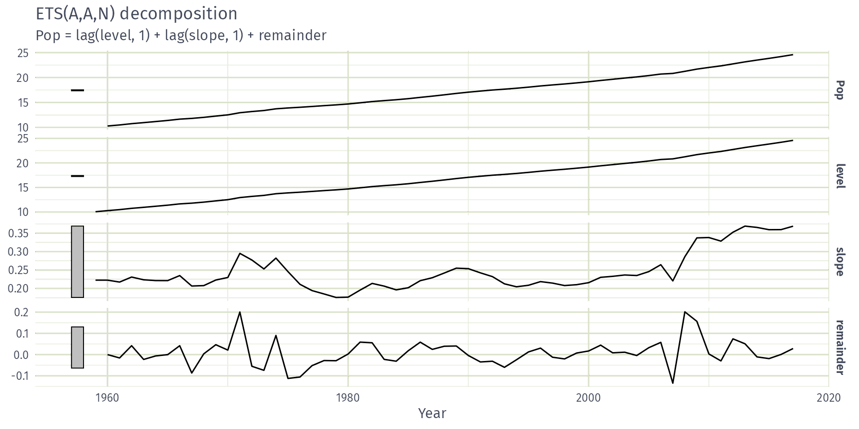
Example: Australian population

components(fit) |> autoplot()

Example: Australian population

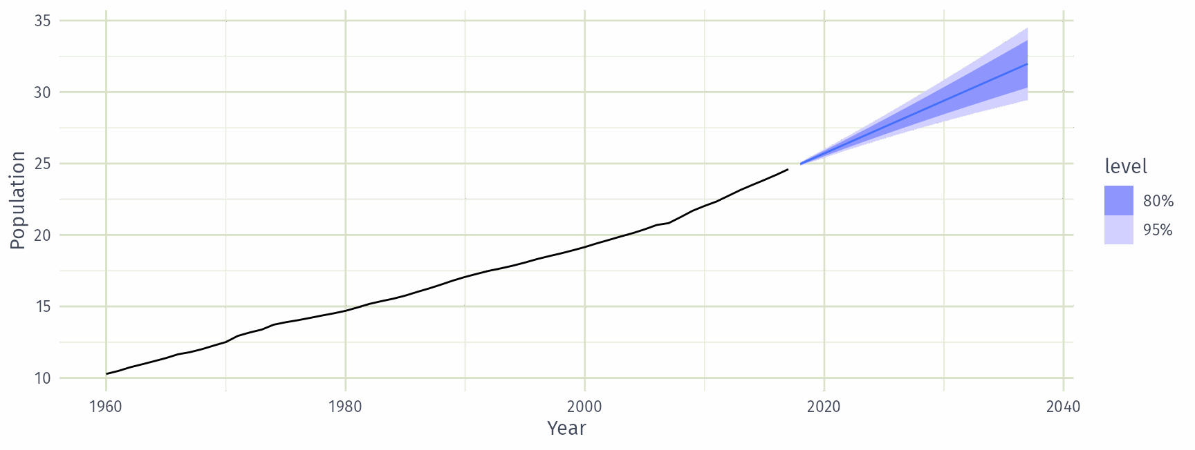
fit |>
  forecast(h = 20) |>
  autoplot(aus_economy) +
  labs(y = "Population", x = "Year")

ETS(A,Ad,N): Damped trend method

Additive errors

\[\begin{aligned} \text{Forecast equation}&& \hat{y}_{T+h|T} &= \ell_T + (\phi + \phi^2 + \cdots + \phi^{h})b_T\\ \text{Measurement equation}&& y_t &= (\ell_{t-1}+\phi b_{t-1})+\varepsilon_t\\ \text{State equations}&& \ell_t&=(\ell_{t-1}+\phi b_{t-1})+\alpha \varepsilon_t\\ && b_t&=\phi b_{t-1}+\beta \varepsilon_t \end{aligned}\]

• Damping parameter \(0<\phi\le 1\).
• If \(\phi=1\), identical to Holt’s linear trend.
• As \(h\rightarrow\infty\), \(\pred{y}{T+h}{T}\rightarrow \ell_T+\phi b_T/(1-\phi)\).
• Short-run forecasts trended, long-run forecasts constant.

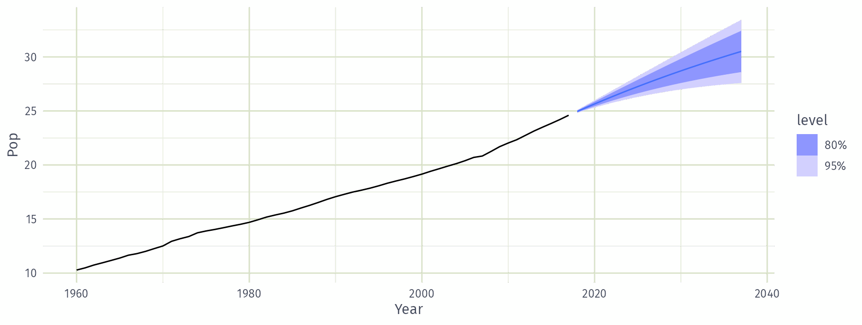
Example: Australian population

aus_economy |>
  model(damped = ETS(Pop ~ error("A") + trend("Ad") + season("N"))) |>
  forecast(h = 20) |>
  autoplot(aus_economy)

Example: Nigerian population

global_economy |>
  filter(Country == "Nigeria") |>
  mutate(Pop = Population / 1e6) |>
  model(
    ANN = ETS(Pop ~ error("A") + trend("N") + season("N")),
    AAN = ETS(Pop ~ error("A") + trend("A") + season("N")),
    AAdN = ETS(Pop ~ error("A") + trend("Ad") + season("N"))
  ) |>
  glance() |>
  select(.model, AICc)

# A tibble: 3 × 2
  .model  AICc
  <chr>  <dbl>
1 ANN    360. 
2 AAN    -37.7
3 AAdN    26.9

Which ETS model is best for Nigeria’s population?

• ETS(A,N,N)
• ETS(A,A,N)
• ETS(A,Ad,N)

Example: National populations

fit <- global_economy |>
  mutate(Pop = Population / 1e6) |>
  model(ets = ETS(Pop))
fit

# A mable: 263 x 2
# Key:     Country [263]
   Country                      ets
   <fct>                    <model>
 1 Afghanistan         <ETS(A,A,N)>
 2 Albania             <ETS(M,A,N)>
 3 Algeria             <ETS(M,A,N)>
 4 American Samoa      <ETS(M,A,N)>
 5 Andorra             <ETS(M,A,N)>
 6 Angola              <ETS(M,A,N)>
 7 Antigua and Barbuda <ETS(M,A,N)>
 8 Arab World          <ETS(M,A,N)>
 9 Argentina           <ETS(A,A,N)>
10 Armenia             <ETS(M,A,N)>
# ℹ 253 more rows

Example: National populations

fit |>
  forecast(h = 5)

# A fable: 1,315 x 5 [1Y]
# Key:     Country, .model [263]
   Country     .model  Year             Pop .mean
   <fct>       <chr>  <dbl>          <dist> <dbl>
 1 Afghanistan ets     2018    N(36, 0.012) 36.4 
 2 Afghanistan ets     2019    N(37, 0.059) 37.3 
 3 Afghanistan ets     2020     N(38, 0.16) 38.2 
 4 Afghanistan ets     2021     N(39, 0.35) 39.0 
 5 Afghanistan ets     2022     N(40, 0.64) 39.9 
 6 Albania     ets     2018 N(2.9, 0.00012)  2.87
 7 Albania     ets     2019   N(2.9, 6e-04)  2.87
 8 Albania     ets     2020  N(2.9, 0.0017)  2.87
 9 Albania     ets     2021  N(2.9, 0.0036)  2.86
10 Albania     ets     2022  N(2.9, 0.0066)  2.86
# ℹ 1,305 more rows

Seasonal methods

ETS(A,A,A): Holt-Winters additive method

\[\begin{aligned} \text{Forecast equation} && \hat{y}_{T+h|T} &= \ell_{T} + hb_{T} + s_{T+h-m(k+1)}\\ \text{Measurement equation}&& y_t&=\ell_{t-1}+b_{t-1}+s_{t-m} + \varepsilon_t\\ \text{State equations}&& \ell_t&=\ell_{t-1}+b_{t-1}+\alpha \varepsilon_t\\ && b_t&=b_{t-1}+\beta \varepsilon_t \\ &&s_t &= s_{t-m} + \gamma\varepsilon_t \end{aligned}\]

• \(k=\) integer part of \((h-1)/m\).
• \(\sum_i s_i \approx 0\).
• Parameters:  \(0\le \alpha\le 1\),  \(0\le \beta\le \alpha\),  \(0\le \gamma\le 1-\alpha\)  and \(m=\) period of seasonality (e.g. \(m=4\) for quarterly data).

ETS(M,A,M): Holt-Winters multiplicative method

\[\begin{aligned} \text{Forecast equation} && \hat{y}_{T+h|T} &= (\ell_{T} + hb_{T}) s_{T+h-m(k+1)}\\ \text{Measurement equation}&& y_t&= (\ell_{t-1}+b_{t-1})s_{t-m}(1 + \varepsilon_t)\\ \text{State equations}&& \ell_t&=(\ell_{t-1}+b_{t-1})(1+\alpha \varepsilon_t)\\ && b_t&=b_{t-1}+\beta(\ell_{t-1}+b_{t-1})\varepsilon_t \\ &&s_t &= s_{t-m}(1 + \gamma\varepsilon_t) \end{aligned}\]

• \(k\) is integer part of \((h-1)/m\).
• \(\sum_i s_i \approx m\).
• Parameters:  \(0\le \alpha\le 1\),  \(0\le \beta\le \alpha\),  \(0\le \gamma\le 1-\alpha\)  and \(m=\) period of seasonality (e.g. \(m=4\) for quarterly data).

Example: Australian holiday tourism

holidays <- tourism |>
  filter(Purpose == "Holiday")
fit <- holidays |> model(ets = ETS(Trips))
fit

# A mable: 76 x 4
# Key:     Region, State, Purpose [76]
   Region         State Purpose          ets
   <chr>          <chr> <chr>        <model>
 1 Adelaide       SA    Holiday <ETS(A,N,A)>
 2 Adelaide Hills SA    Holiday <ETS(A,A,N)>
 3 Alice Springs  NT    Holiday <ETS(M,N,A)>
 4 Ballarat       VIC   Holiday <ETS(M,N,A)>
 5 Barkly         NT    Holiday <ETS(A,N,A)>
 6 Barossa        SA    Holiday <ETS(A,N,N)>
 7 Bendigo Loddon VIC   Holiday <ETS(M,N,N)>
 8 Blue Mountains NSW   Holiday <ETS(M,N,M)>
 9 Brisbane       QLD   Holiday <ETS(A,A,N)>
10 Bundaberg      QLD   Holiday <ETS(A,N,A)>
# ℹ 66 more rows

Example: Australian holiday tourism

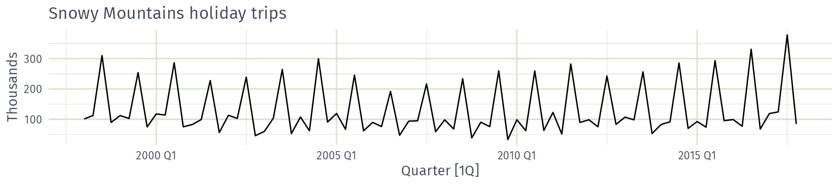
Which ETS model suits Snowy Mountains holiday trips?

• ETS(?,A,A)
• ETS(?,N,A)
• ETS(?,N,M)
• ETS(?,N,N)

Example: Australian holiday tourism

fit |>
  filter(Region == "Snowy Mountains") |>
  report()

Series: Trips 
Model: ETS(M,N,A) 
  Smoothing parameters:
    alpha = 0.157 
    gamma = 1e-04 

  Initial states:
 l[0] s[0] s[-1] s[-2] s[-3]
  142  -61   131 -42.2 -27.7

  sigma^2:  0.0388

 AIC AICc  BIC 
 852  854  869 

Example: Australian holiday tourism

fit |>
  filter(Region == "Snowy Mountains") |>
  components()

# A dable: 84 x 9 [1Q]
# Key:     Region, State, Purpose, .model [1]
# :        Trips = (lag(level, 1) + lag(season, 4)) * (1 + remainder)
   Region          State Purpose .model Quarter Trips level season remainder
   <chr>           <chr> <chr>   <chr>    <qtr> <dbl> <dbl>  <dbl>     <dbl>
 1 Snowy Mountains NSW   Holiday ets    1997 Q1  NA     NA   -27.7   NA     
 2 Snowy Mountains NSW   Holiday ets    1997 Q2  NA     NA   -42.2   NA     
 3 Snowy Mountains NSW   Holiday ets    1997 Q3  NA     NA   131.    NA     
 4 Snowy Mountains NSW   Holiday ets    1997 Q4  NA    142.  -61.0   NA     
 5 Snowy Mountains NSW   Holiday ets    1998 Q1 101.   140.  -27.7   -0.113 
 6 Snowy Mountains NSW   Holiday ets    1998 Q2 112.   142.  -42.2    0.154 
 7 Snowy Mountains NSW   Holiday ets    1998 Q3 310.   148.  131.     0.137 
 8 Snowy Mountains NSW   Holiday ets    1998 Q4  89.8  148.  -61.0    0.0335
 9 Snowy Mountains NSW   Holiday ets    1999 Q1 112.   147.  -27.7   -0.0687
10 Snowy Mountains NSW   Holiday ets    1999 Q2 103.   147.  -42.2   -0.0199
# ℹ 74 more rows

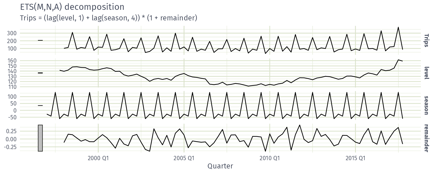
Example: Australian holiday tourism

fit |>
  filter(Region == "Snowy Mountains") |>
  components() |>
  autoplot()

Example: Australian holiday tourism

fit |> forecast()

# A fable: 608 x 7 [1Q]
# Key:     Region, State, Purpose, .model [76]
   Region         State Purpose .model Quarter       Trips .mean
   <chr>          <chr> <chr>   <chr>    <qtr>      <dist> <dbl>
 1 Adelaide       SA    Holiday ets    2018 Q1 N(210, 457) 210. 
 2 Adelaide       SA    Holiday ets    2018 Q2 N(173, 473) 173. 
 3 Adelaide       SA    Holiday ets    2018 Q3 N(169, 489) 169. 
 4 Adelaide       SA    Holiday ets    2018 Q4 N(186, 505) 186. 
 5 Adelaide       SA    Holiday ets    2019 Q1 N(210, 521) 210. 
 6 Adelaide       SA    Holiday ets    2019 Q2 N(173, 537) 173. 
 7 Adelaide       SA    Holiday ets    2019 Q3 N(169, 553) 169. 
 8 Adelaide       SA    Holiday ets    2019 Q4 N(186, 569) 186. 
 9 Adelaide Hills SA    Holiday ets    2018 Q1   N(19, 36)  19.4
10 Adelaide Hills SA    Holiday ets    2018 Q2   N(20, 36)  19.6
# ℹ 598 more rows

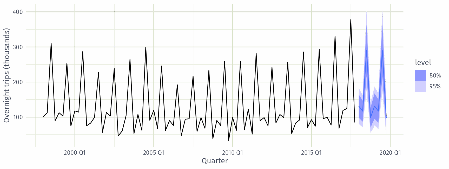
Example: Australian holiday tourism

fit |>
  forecast() |>
  filter(Region == "Snowy Mountains") |>
  autoplot(holidays) +
  labs(x = "Quarter", y = "Overnight trips (thousands)")

ETS taxonomy

Exponential smoothing models

Additive Error		N	A	M
Trend Component		(None)	(Additive)	(Multiplicative)
N	(None)	A,N,N	A,N,A	A,N,M
A	(Additive)	A,A,N	A,A,A	A,A,M
A\(_\text{d}\)	(Additive damped)	A,A\(_\text{d}\),N	A,A\(_\text{d}\),A	A,A\(_\text{d}\),M

Multiplicative Error		N	A	M
Trend Component		(None)	(Additive)	(Multiplicative)
N	(None)	M,N,N	M,N,A	M,N,M
A	(Additive)	M,A,N	M,A,A	M,A,M
A\(_\text{d}\)	(Additive damped)	M,A\(_\text{d}\),N	M,A\(_\text{d}\),A	M,A\(_\text{d}\),M

Estimating ETS models

• Smoothing parameters \(\alpha\), \(\beta\), \(\gamma\) and \(\phi\), and the initial states \(\ell_0\), \(b_0\), \(s_0,s_{-1},\dots,s_{-m+1}\) are estimated by maximising the “likelihood” = the probability of the data arising from the specified model.
• For models with additive errors equivalent to minimising SSE.
• For models with multiplicative errors, not equivalent to minimising SSE.

Model selection

Akaike’s Information Criterion

\[\text{AIC} = -2\log(L) + 2k\]

where \(L\) is the likelihood and \(k\) is the number of parameters and initial states estimated in the model.

Corrected AIC

\[\text{AIC}_{\text{c}} = \text{AIC} + \frac{2k(k+1)}{T-k-1}\]

which is the AIC corrected (for small sample bias).

Bayesian Information Criterion

\[\text{BIC} = \text{AIC} + k(\log(T)-2).\]

AIC and cross-validation

Minimising the AIC assuming Gaussian residuals is asymptotically equivalent to minimising one-step time series cross validation MSE.

Time series cross-validation is covered on Day 5.

Automatic forecasting

From Hyndman et al. (IJF, 2002):

1. Apply each model that is appropriate to the data. Optimise parameters and initial values using MLE.
2. Select best method using AICc.
3. Produce forecasts using best method.
4. Obtain forecast intervals using underlying state space model.

• Method performed very well in M3 competition.
• Used as a benchmark in the M4 competition.

Non-Gaussian forecast distributions

Non-Gaussian forecast distributions

vic_cafe <- aus_retail |>
  filter(State == "Victoria",
         Industry == "Cafes, restaurants and catering services") |>
  select(Month, Turnover)
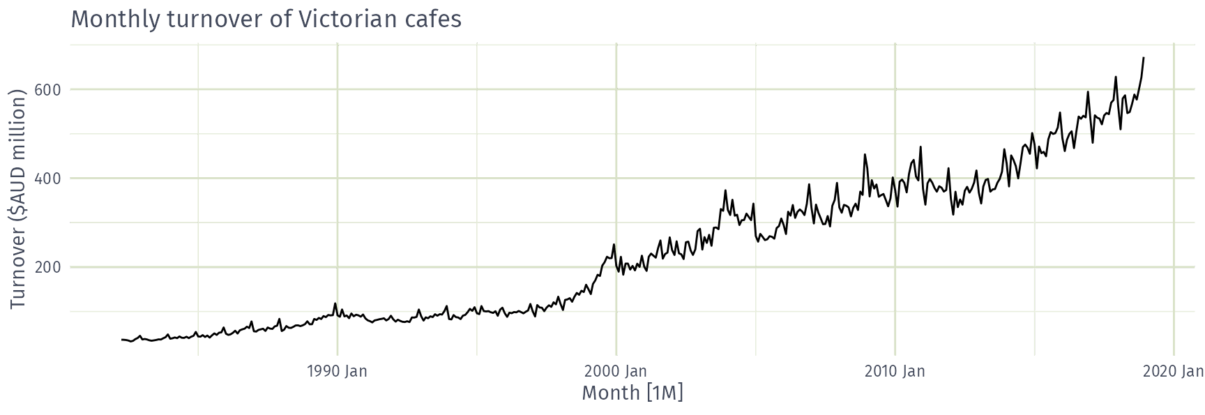
vic_cafe |>
  autoplot(Turnover) +
  labs(title = "Monthly turnover of Victorian cafes", y = "Turnover ($AUD million)")

Forecasting with transformations

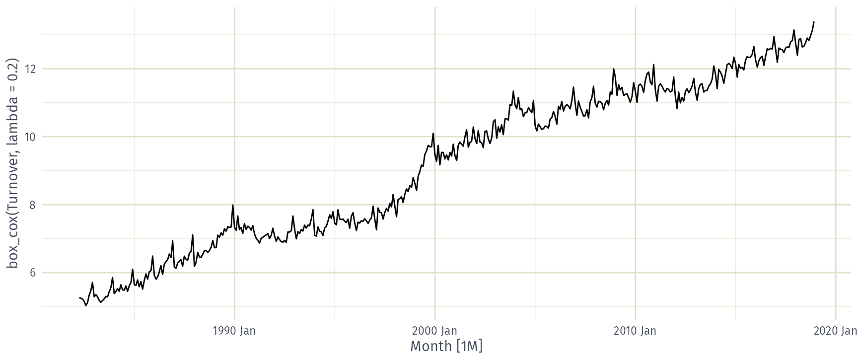
vic_cafe |> autoplot(box_cox(Turnover, lambda = 0.2))

Forecasting with transformations

vic_cafe |>
  model(
    raw = ETS(Turnover),
    log = ETS(log(Turnover))
  ) |>
  glance() |>
  select(.model, AICc)

# A tibble: 2 × 2
  .model   AICc
  <chr>   <dbl>
1 raw    4613. 
2 log      82.8

Which model is better for Victorian cafe turnover?

• ETS(log(Turnover))
• ETS(Turnover)
• Can’t tell from AICc

Forecasting with transformations

fit <- vic_cafe |>
  model(ets = ETS(box_cox(Turnover, 0.2)))
fit

# A mable: 1 x 1
           ets
       <model>
1 <ETS(A,A,A)>

(fc <- fit |> forecast(h = "3 years"))

# A fable: 36 x 4 [1M]
# Key:     .model [1]
   .model    Month        Turnover .mean
   <chr>     <mth>          <dist> <dbl>
 1 ets    2019 Jan  t(N(13, 0.02))  608.
 2 ets    2019 Feb t(N(13, 0.028))  563.
 3 ets    2019 Mar t(N(13, 0.036))  629.
 4 ets    2019 Apr t(N(13, 0.044))  615.
 5 ets    2019 May t(N(13, 0.052))  613.
 6 ets    2019 Jun t(N(13, 0.061))  593.
 7 ets    2019 Jul t(N(13, 0.069))  624.
 8 ets    2019 Aug t(N(13, 0.077))  640.
 9 ets    2019 Sep t(N(13, 0.085))  630.
10 ets    2019 Oct t(N(13, 0.093))  642.
# ℹ 26 more rows

• t(N) denotes a transformed normal distribution.
• The distribution is back-transformed and the mean (.mean) is bias-adjusted automatically.

Forecasting with transformations

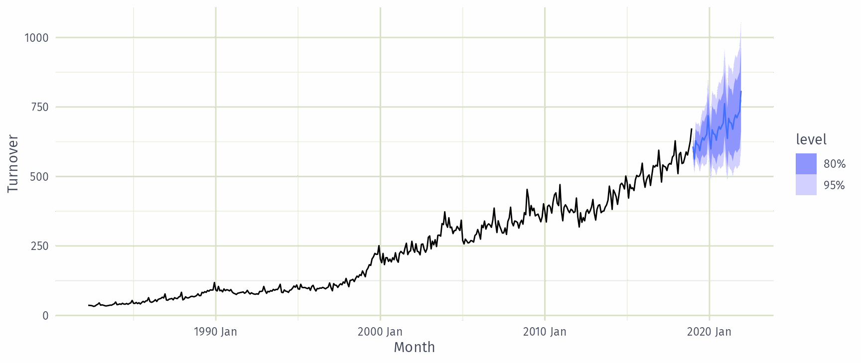
fc |> autoplot(vic_cafe)

Bootstrapped forecast distributions

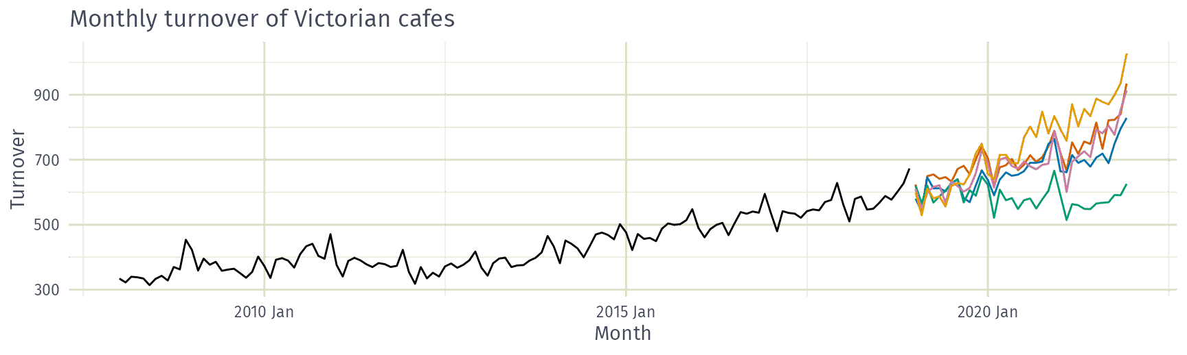
sim <- fit |> generate(h = "3 years", times = 5, bootstrap = TRUE)
sim

# A tsibble: 180 x 4 [1M]
# Key:       .model, .rep [5]
   .model    Month .rep   .sim
   <chr>     <mth> <chr> <dbl>
 1 ets    2019 Jan 1      624.
 2 ets    2019 Feb 1      541.
 3 ets    2019 Mar 1      649.
 4 ets    2019 Apr 1      655.
 5 ets    2019 May 1      641.
 6 ets    2019 Jun 1      646.
 7 ets    2019 Jul 1      633.
 8 ets    2019 Aug 1      671.
 9 ets    2019 Sep 1      681.
10 ets    2019 Oct 1      655.
# ℹ 170 more rows

Bootstrapped forecast distributions

vic_cafe |>
  filter(year(Month) >= 2008) |>
  ggplot(aes(x = Month)) +
  geom_line(aes(y = Turnover)) +
  geom_line(aes(y = .sim, colour = as.factor(.rep)), data = sim) +
  labs(title = "Monthly turnover of Victorian cafes") +
  guides(colour = "none")

Bootstrapped forecast distributions

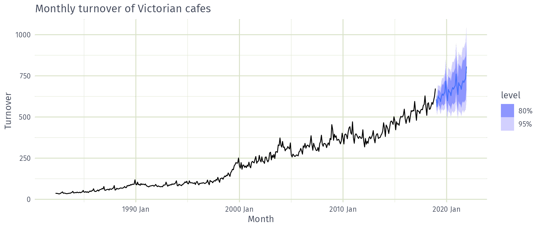
fc <- fit |> forecast(h = "3 years", bootstrap = TRUE)
fc

# A fable: 36 x 4 [1M]
# Key:     .model [1]
   .model    Month     Turnover .mean
   <chr>     <mth>       <dist> <dbl>
 1 ets    2019 Jan sample[5000]  608.
 2 ets    2019 Feb sample[5000]  563.
 3 ets    2019 Mar sample[5000]  629.
 4 ets    2019 Apr sample[5000]  615.
 5 ets    2019 May sample[5000]  613.
 6 ets    2019 Jun sample[5000]  593.
 7 ets    2019 Jul sample[5000]  624.
 8 ets    2019 Aug sample[5000]  640.
 9 ets    2019 Sep sample[5000]  631.
10 ets    2019 Oct sample[5000]  642.
# ℹ 26 more rows

Bootstrapped forecast distributions

fc |> autoplot(vic_cafe) +
  labs(title = "Monthly turnover of Victorian cafes")