AFRICAST

Tidy time series & forecasting in R

ARIMA models

Session 6 of 10

workshop.f4sg.org/africastForecasting for Social Good

ARIMA models

ARIMA models

ARIMA models describe the autocorrelations in the data: how each observation relates to past observations and past errors.

An ARIMA model is rarely interpretable in terms of visible data structures like trend and seasonality. But it can capture a huge range of time series patterns.

Stationarity

Definition

If \(\{y_t\}\) is a stationary time series, then for all \(s\), the distribution of \((y_t,\dots,y_{t+s})\) does not depend on \(t\).

A stationary series is:

• roughly horizontal
• constant variance
• no patterns predictable in the long-term

Stationary?

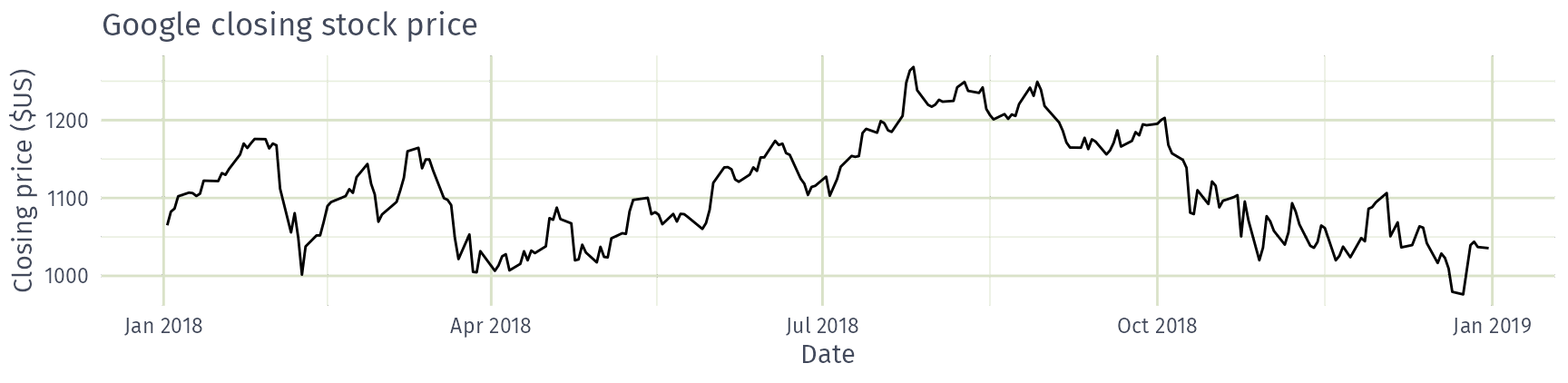
Is the Google closing stock price stationary?

• Yes
• No

Stationary?

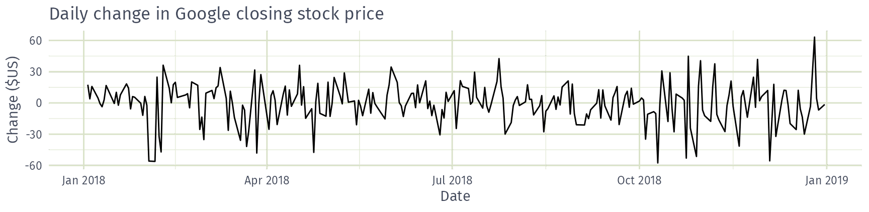
Is the daily change in Google closing stock price stationary?

• Yes
• No

Random walks

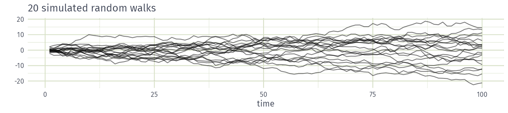
A random walk, \(y_t = y_{t-1} + \varepsilon_t\) with white noise \(\varepsilon_t\), has no trend or seasonality.

Is a random walk stationary?

• Yes
• No

Differencing

Differences

First difference: \(y'_t = y_t - y_{t-1}\)

Second difference: \(y''_t = y'_t - y'_{t-1} = y_t - 2y_{t-1} + y_{t-2}\)

Seasonal difference: \(y_t - y_{t-m}\), where \(m\) is the seasonal period

• Differencing helps to stabilise the mean.
• A random walk is not stationary (its variance grows over time), but its first difference is white noise, which is stationary. The Google stock price behaves like a random walk.
• Occasionally a second difference is needed; it is almost never necessary to go further.

Autoregressive models

Autoregressive (AR) models

\[ y_{t} = c + \phi_{1}y_{t - 1} + \phi_{2}y_{t - 2} + \cdots + \phi_{p}y_{t - p} + \varepsilon_{t}, \] where \(\varepsilon_t\) is white noise. A multiple regression with lagged values of \(y_t\) as predictors.

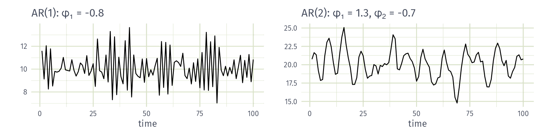
• Cyclic behaviour is possible when \(p\ge 2\).

Moving average models

Moving average (MA) models

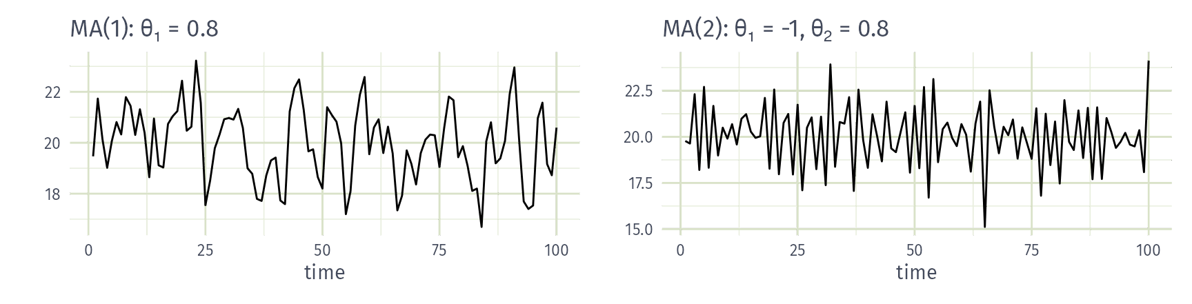
\[ y_{t} = c + \varepsilon_t + \theta_{1}\varepsilon_{t - 1} + \theta_{2}\varepsilon_{t - 2} + \cdots + \theta_{q}\varepsilon_{t - q}, \] where \(\varepsilon_t\) is white noise. A multiple regression with lagged errors as predictors. Don’t confuse with moving average smoothing!

ARIMA models

Autoregressive moving average (ARMA) models

\[\begin{aligned} y_{t} &= c + \phi_{1}y_{t - 1} + \cdots + \phi_{p}y_{t - p} \\ & \qquad + \theta_{1}\varepsilon_{t - 1} + \cdots + \theta_{q}\varepsilon_{t - q} + \varepsilon_{t}. \end{aligned}\]

• Predictors include both lagged values of \(y_t\) and lagged errors.

Autoregressive integrated moving average models

• Combine ARMA model with differencing.
• \(d\)-differenced series follows an ARMA model.
• Need to choose \(p\), \(d\), \(q\) and whether or not to include \(c\).

ARIMA models

ARIMA(\(p, d, q\)) model

AR:	\(p =\) order of the autoregressive part
I:	\(d =\) degree of first differencing involved
MA:	\(q =\) order of the moving average part.

• White noise model: ARIMA(0,0,0)
• Random walk: ARIMA(0,1,0) with no constant
• Random walk with drift: ARIMA(0,1,0) with const.
• AR(\(p\)): ARIMA(\(p\),0,0)
• MA(\(q\)): ARIMA(0,0,\(q\))

Example: National populations

fit_pop <- global_economy |>
  model(arima = ARIMA(Population))
fit_pop

# A mable: 263 x 2
# Key:     Country [263]
   Country                               arima
   <fct>                               <model>
 1 Afghanistan                  <ARIMA(4,2,1)>
 2 Albania                      <ARIMA(0,2,2)>
 3 Algeria                      <ARIMA(2,2,2)>
 4 American Samoa               <ARIMA(2,2,2)>
 5 Andorra             <ARIMA(2,1,2) w/ drift>
 6 Angola                       <ARIMA(4,2,1)>
 7 Antigua and Barbuda <ARIMA(2,1,2) w/ drift>
 8 Arab World                   <ARIMA(0,2,1)>
 9 Argentina                    <ARIMA(2,2,2)>
10 Armenia                      <ARIMA(3,2,0)>
# ℹ 253 more rows

Example: National populations

fit_pop |>
  filter(Country == "Australia") |>
  report()

Series: Population 
Model: ARIMA(0,2,1) 

Coefficients:
         ma1
      -0.661
s.e.   0.107

sigma^2 estimated as 4.063e+09:  log likelihood=-699
AIC=1401   AICc=1402   BIC=1405

With \(d=2\) the MA(1) model is for the second differences \(y_t - 2y_{t-1} + y_{t-2}\), so \[y_t = 2y_{t-1} - y_{t-2} - 0.661 \varepsilon_{t-1} + \varepsilon_t, \qquad \varepsilon_t \sim \text{NID}(0, 4.06\times10^9)\]

Understanding ARIMA models

\(c\) is the constant in the ARMA model for the \(d\)-times differenced series.

• If \(c=0\) and \(d=0\), the long-term forecasts will go to zero.
• If \(c=0\) and \(d=1\), the long-term forecasts will go to a non-zero constant.
• If \(c=0\) and \(d=2\), the long-term forecasts will follow a straight line.
• If \(c\ne0\) and \(d=0\), the long-term forecasts will go to the mean of the data.
• If \(c\ne0\) and \(d=1\), the long-term forecasts will follow a straight line.
• If \(c\ne0\) and \(d=2\), the long-term forecasts will follow a quadratic trend.

Example: National populations

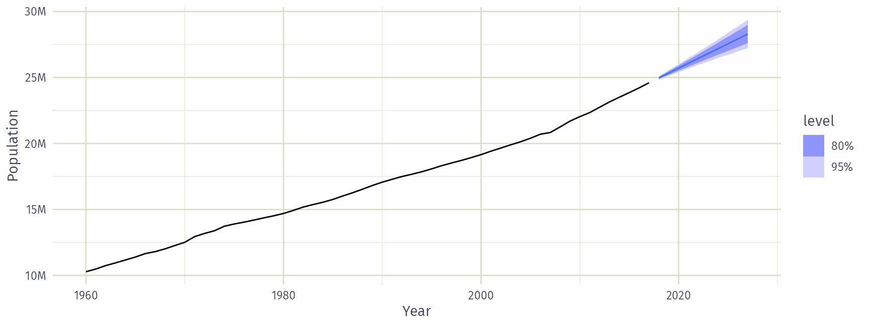
Australia’s population model is ARIMA(0,2,1) with no constant. What shape will its long-term forecasts take?

• Flat line
• Straight line
• Quadratic curve
• Decay to zero

Understanding ARIMA models

Forecast variance and \(d\)

• The higher the value of \(d\), the more rapidly the prediction intervals increase in size.
• For \(d=0\), the long-term forecast standard deviation will go to the standard deviation of the historical data.

Example: National populations

fit_pop |>
  forecast(h = 10) |>
  filter(Country == "Australia") |>
  autoplot(global_economy) +
  scale_y_continuous(labels = scales::label_number(scale = 1e-6, suffix = "M"))

How does ARIMA() work?

Hyndman and Khandakar (JSS, 2008) algorithm

• Select the number of seasonal differences \(D\) via a seasonal strength test, then the number of differences \(d\) via KPSS tests.
• Select \(p\), \(q\) (and \(P\), \(Q\) for seasonal models) and inclusion of \(c\) by minimising AICc.
• Use stepwise search to traverse model space.

How does ARIMA() work?

\[\text{AICc} = -2 \log(L) + 2(p+q+k+1)\left[1 + \frac{(p+q+k+2)}{T-p-q-k-2}\right]\] where \(L\) is the maximised likelihood fitted to the differenced data, \(k=1\) if \(c\neq 0\) and \(k=0\) otherwise.

Can you choose between ARIMA(2,1,0) and ARIMA(1,0,1) by comparing their AICc?

• Yes
• No

How does ARIMA() work?

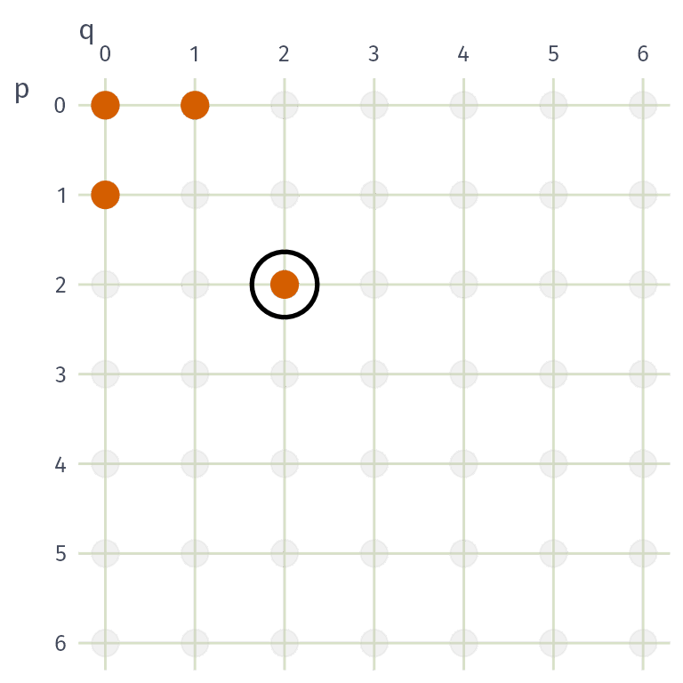
1. Fit ARIMA\((2,d,2)\), ARIMA\((0,d,0)\), ARIMA\((1,d,0)\) and ARIMA\((0,d,1)\). The lowest AICc becomes the current model.
2. Fit variations of the current model: vary \(p\), \(q\) or both by \(\pm1\), and include/exclude \(c\). The lowest AICc becomes the current model.
3. Repeat step 2 until no lower AICc can be found.

Is this search guaranteed to find the model with the lowest AICc?

• Yes
• No

How does ARIMA() work?

Step 1: fit the four starting models.

ARIMA\((2,d,2)\) has the lowest AICc, so it becomes the current model (circled).

How does ARIMA() work?

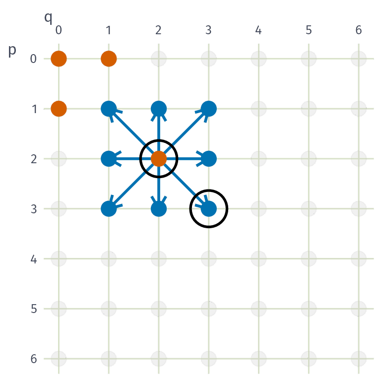
Step 2: fit the neighbours of ARIMA\((2,d,2)\).

ARIMA\((3,d,3)\) has a lower AICc, so it becomes the current model.

How does ARIMA() work?

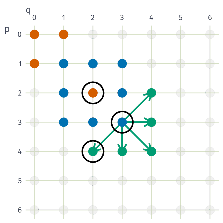
Step 2 (repeated): fit the neighbours of ARIMA\((3,d,3)\).

ARIMA\((4,d,2)\) has a lower AICc, so it becomes the current model.

How does ARIMA() work?

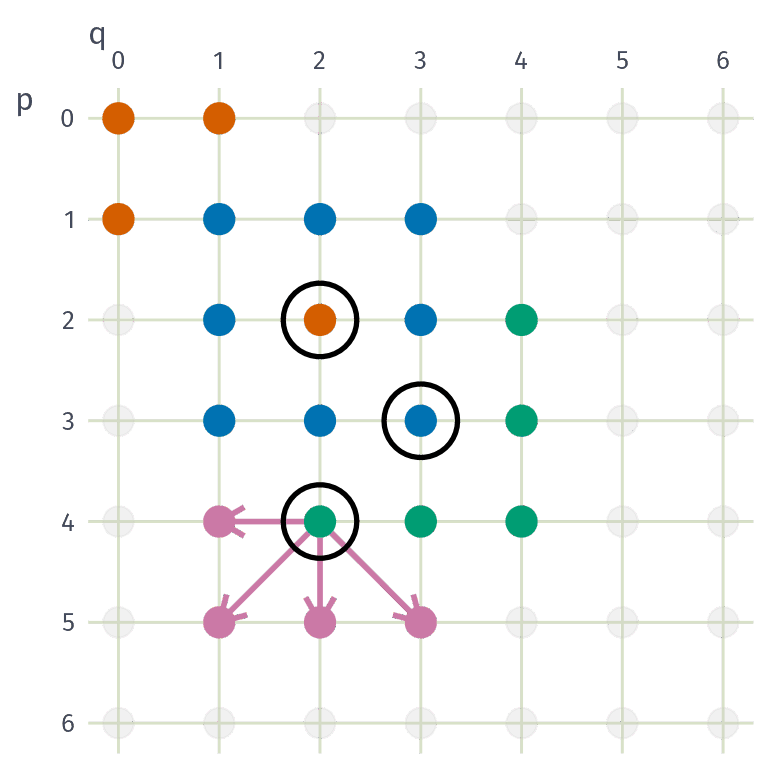
Step 2 (repeated): fit the neighbours of ARIMA\((4,d,2)\).

None has a lower AICc, so the search stops and ARIMA\((4,d,2)\) is selected.

The search is local, so a model with a lower AICc may exist elsewhere in the grid.

Seasonal ARIMA models

Seasonal ARIMA models

\[\text{ARIMA}~\underbrace{(p,d,q)}_{\text{Non-seasonal part}}~\underbrace{(P,D,Q)_m}_{\text{Seasonal part}}\]

• \(m =\) seasonal period (e.g. 12 for monthly data, 4 for quarterly data).
• \(d\) first differences, \(D\) seasonal differences
• \(p\) AR order, \(q\) MA order
• \(P\) seasonal AR order, \(Q\) seasonal MA order

Seasonal and non-seasonal terms combine multiplicatively

Corticosteroid drug sales

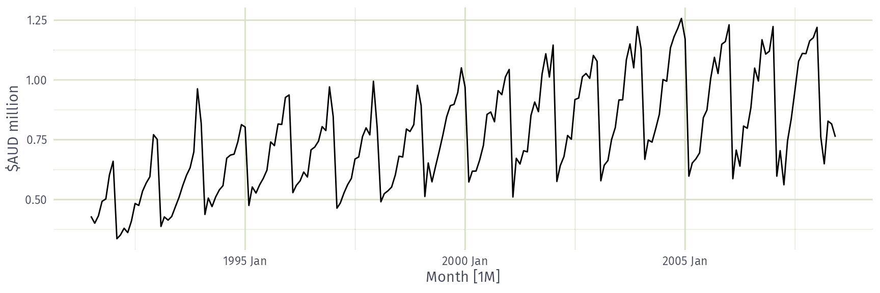
Monthly Australian Pharmaceutical Benefits Scheme (PBS) expenditure on corticosteroid (H02) drugs.

h02 <- PBS |>
  filter(ATC2 == "H02") |>
  summarise(Cost = sum(Cost) / 1e6)
h02 |> autoplot(Cost) + labs(y = "$AUD million")

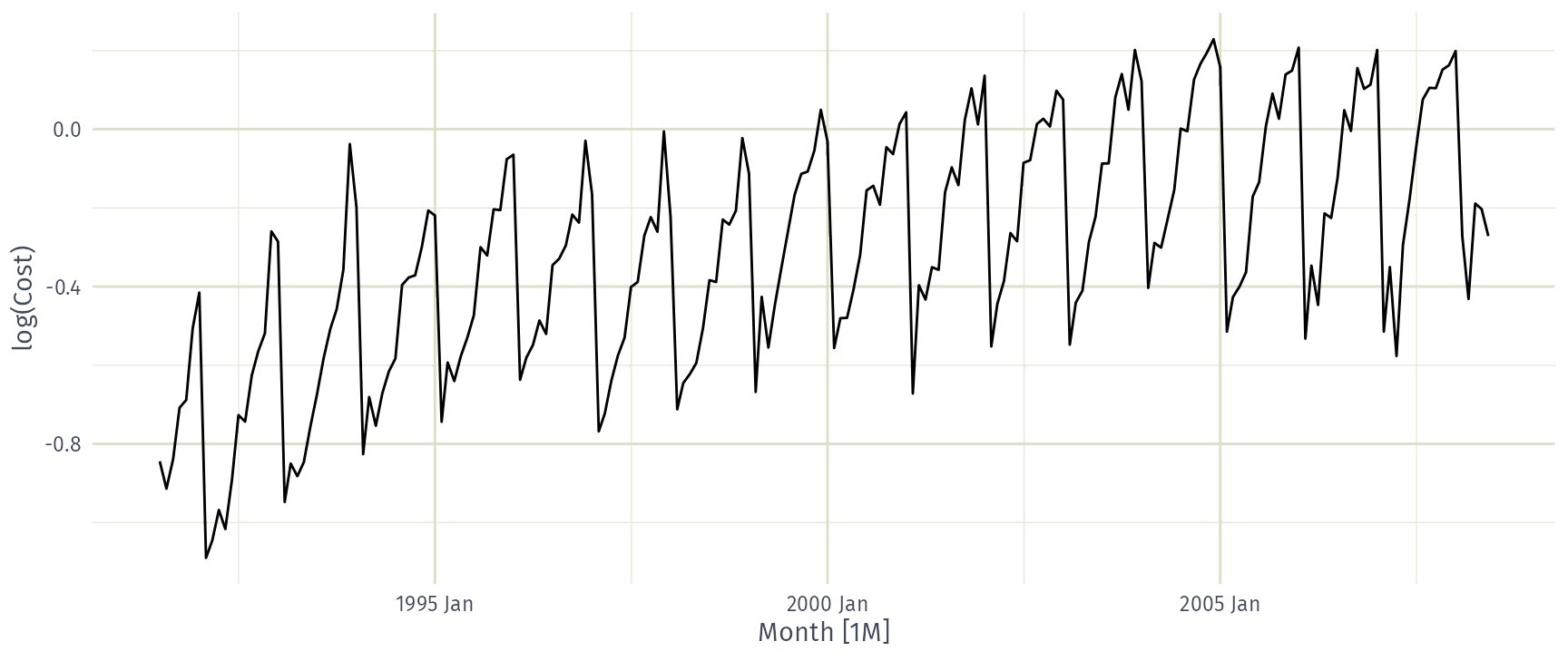
Corticosteroid drug sales: log transform

h02 |> autoplot(log(Cost))

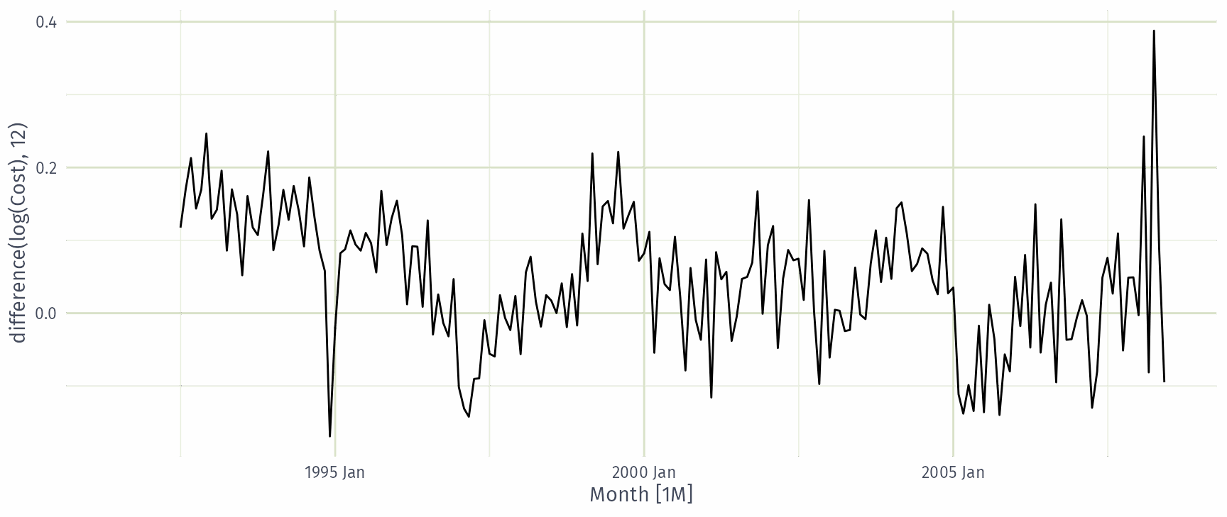
Corticosteroid drug sales: seasonal difference

h02 |> autoplot(log(Cost) |> difference(12))

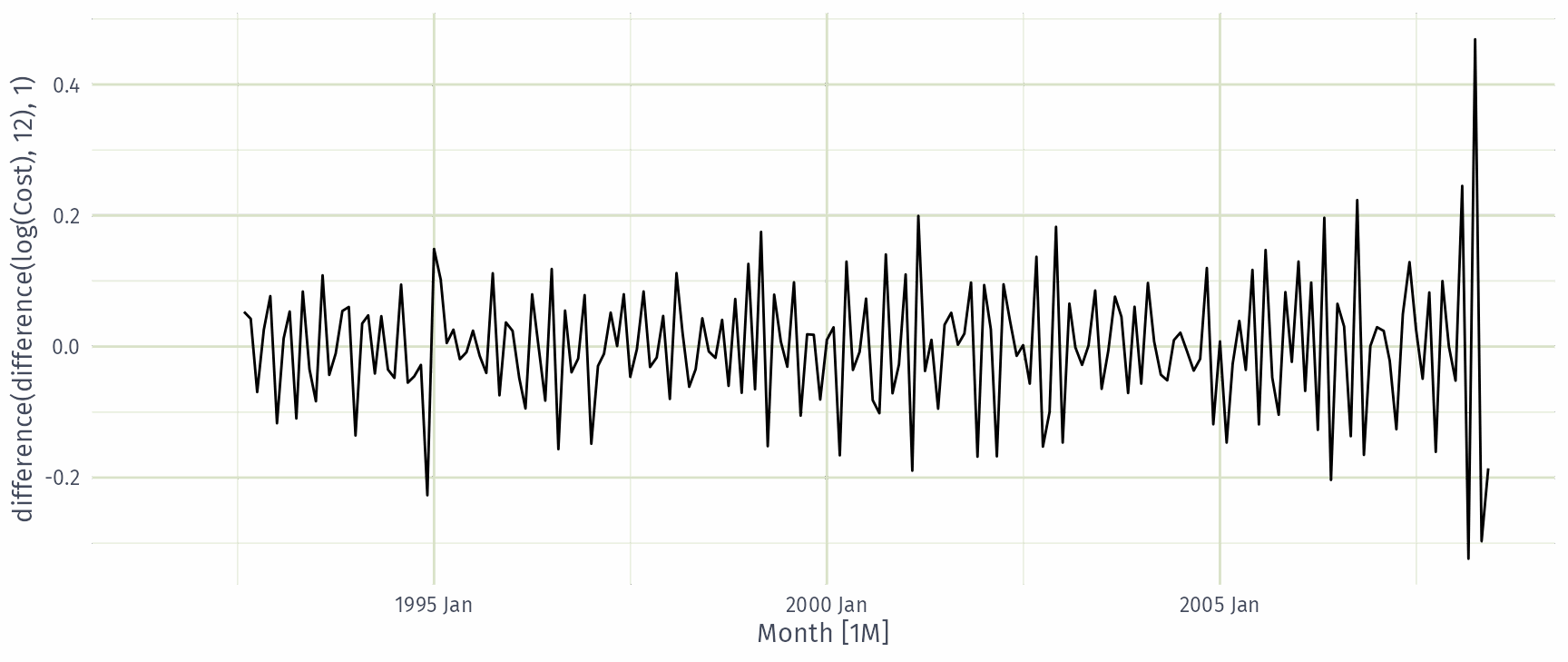
Corticosteroid drug sales: seasonal and first difference

h02 |> autoplot(log(Cost) |> difference(12) |> difference(1))

Corticosteroid drug sales: automatic ARIMA

fit_h02 <- h02 |>
  model(auto = ARIMA(log(Cost)))
fit_h02 |> report()

Series: Cost 
Model: ARIMA(2,1,0)(0,1,1)[12] 
Transformation: log(Cost) 

Coefficients:
          ar1      ar2     sma1
      -0.8491  -0.4207  -0.6401
s.e.   0.0712   0.0714   0.0694

sigma^2 estimated as 0.004387:  log likelihood=245
AIC=-483   AICc=-483   BIC=-470

\(d=1\) and \(D=1\) match the differencing above, leaving an AR(2) and a seasonal MA(1) at lag 12.

Corticosteroid drug sales: manual ARIMA

Specify the orders with pdq() and PDQ(), and the constant with 0 + (exclude) or 1 + (include).

h02 |>
  model(manual = ARIMA(log(Cost) ~ 0 + pdq(2, 1, 0) + PDQ(0, 1, 1))) |>
  report()

Series: Cost 
Model: ARIMA(2,1,0)(0,1,1)[12] 
Transformation: log(Cost) 

Coefficients:
          ar1      ar2     sma1
      -0.8491  -0.4207  -0.6401
s.e.   0.0712   0.0714   0.0694

sigma^2 estimated as 0.004387:  log likelihood=245
AIC=-483   AICc=-483   BIC=-470

Orders can be chosen manually by inspecting the ACF and PACF of the differenced data.

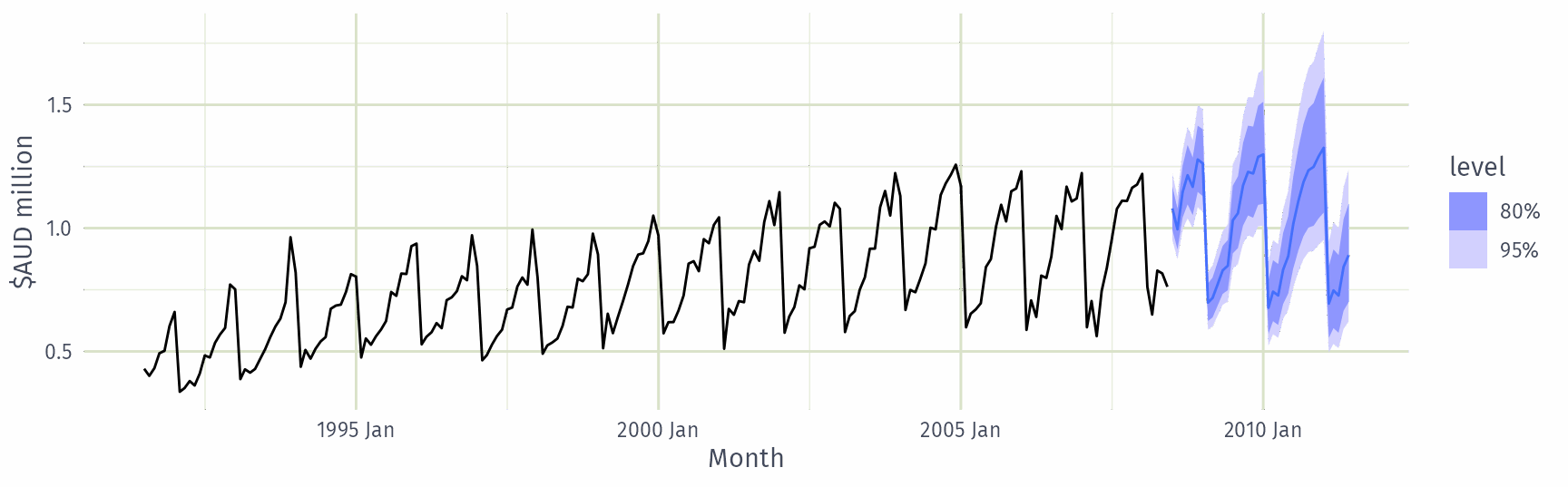
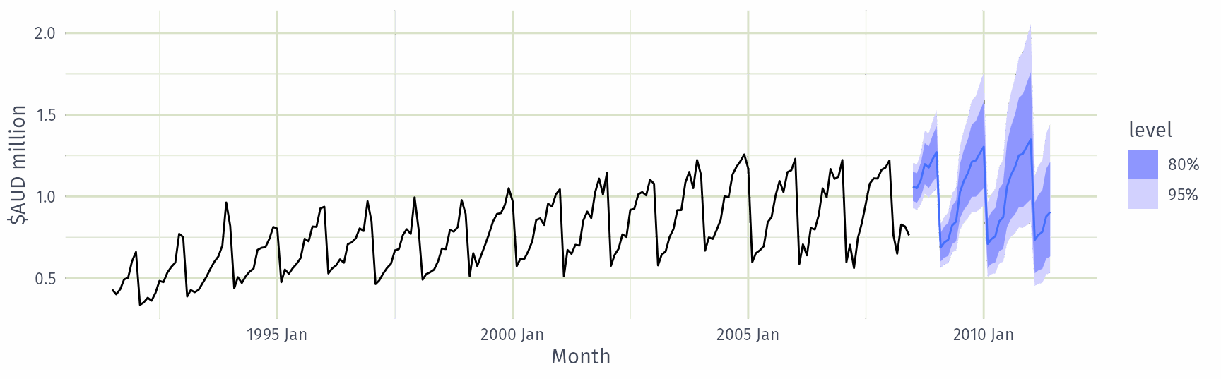
Corticosteroid drug sales: forecasts

fit_h02 |>
  forecast(h = "3 years") |>
  autoplot(h02) +
  labs(y = "$AUD million")

Corticosteroid drug sales: searching harder

By default ARIMA() takes shortcuts to keep model selection fast.

Search options

• stepwise = FALSE: fit every model within the order limit, not just the stepwise path.
• approximation = FALSE: estimate with the exact likelihood rather than an approximation.
• order_constraint: limit the total number of AR and MA terms considered.

A wider search is slower, but may find a model with a lower AICc.

Corticosteroid drug sales: searching harder

fit_h02_best <- h02 |>
  model(best = ARIMA(log(Cost),
    stepwise = FALSE,
    approximation = FALSE,
    order_constraint = p + q + P + Q <= 9
  ))
fit_h02_best |> report()

Series: Cost 
Model: ARIMA(4,1,1)(2,1,2)[12] 
Transformation: log(Cost) 

Coefficients:
          ar1    ar2    ar3     ar4     ma1   sar1    sar2    sma1   sma2
      -0.0425  0.210  0.202  -0.227  -0.742  0.621  -0.383  -1.202  0.496
s.e.   0.2167  0.181  0.114   0.081   0.207  0.242   0.118   0.249  0.213

sigma^2 estimated as 0.004049:  log likelihood=254
AIC=-489   AICc=-487   BIC=-456

Same differencing and transformation, so the AICc is comparable: \(-487\) vs \(-483\) for the automatic model, using nine coefficients instead of three.

Corticosteroid drug sales: residuals

gg_tsresiduals(fit_h02_best, lag_max = 36)

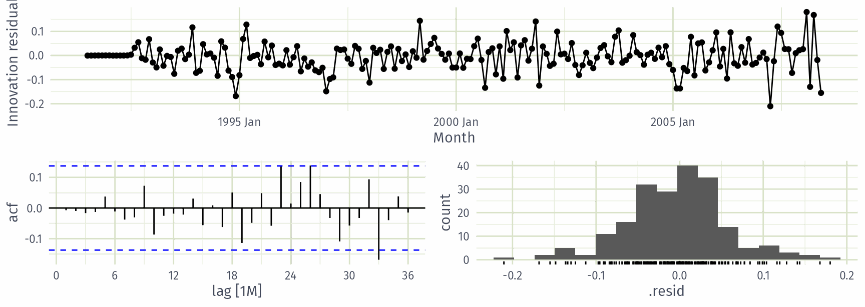
Corticosteroid drug sales: residuals

Ljung-Box tests (from the regression session), with dof set to the number of estimated coefficients.

bind_rows(
  augment(fit_h02) |> features(.innov, ljung_box, lag = 36, dof = 3),
  augment(fit_h02_best) |> features(.innov, ljung_box, lag = 36, dof = 9)
)

# A tibble: 2 × 3
  .model lb_stat lb_pvalue
  <chr>    <dbl>     <dbl>
1 auto      59.3   0.00332
2 best      36.5   0.106  

The automatic model leaves autocorrelation in its residuals; the wider search does not, so we prefer it.

Corticosteroid drug sales: forecasts

fit_h02_best |>
  forecast(h = "3 years") |>
  autoplot(h02) +
  labs(y = "$AUD million")