
AFRICASTTidy time series & forecasting in R
Session 4 of 10
What do you forecast (or wish you could) in your work?
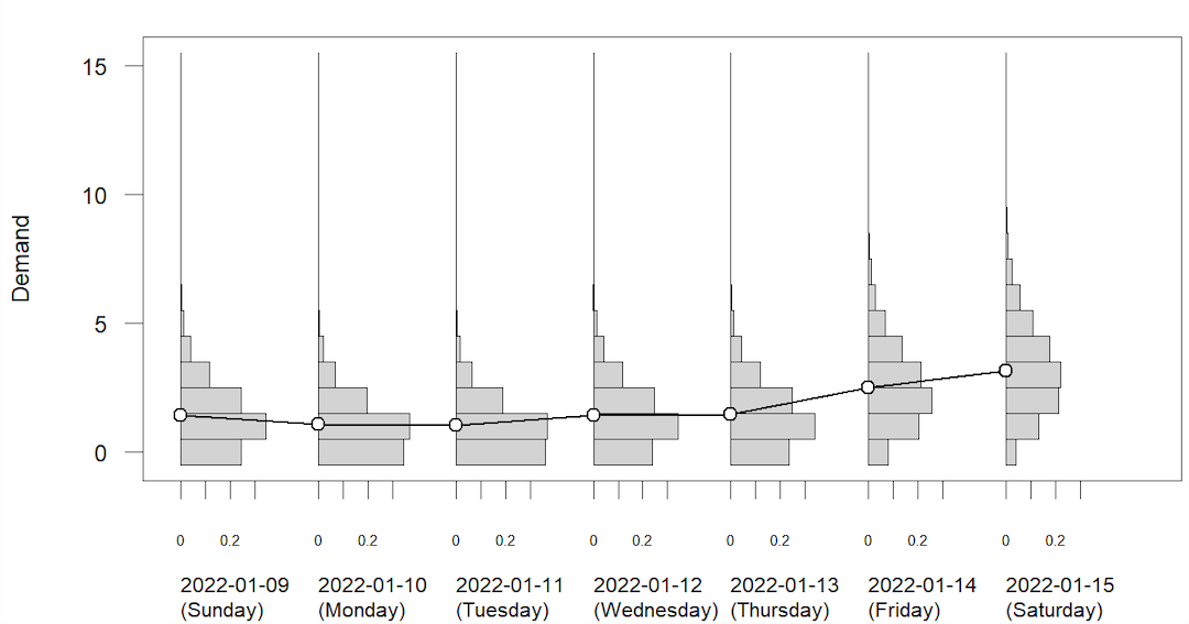
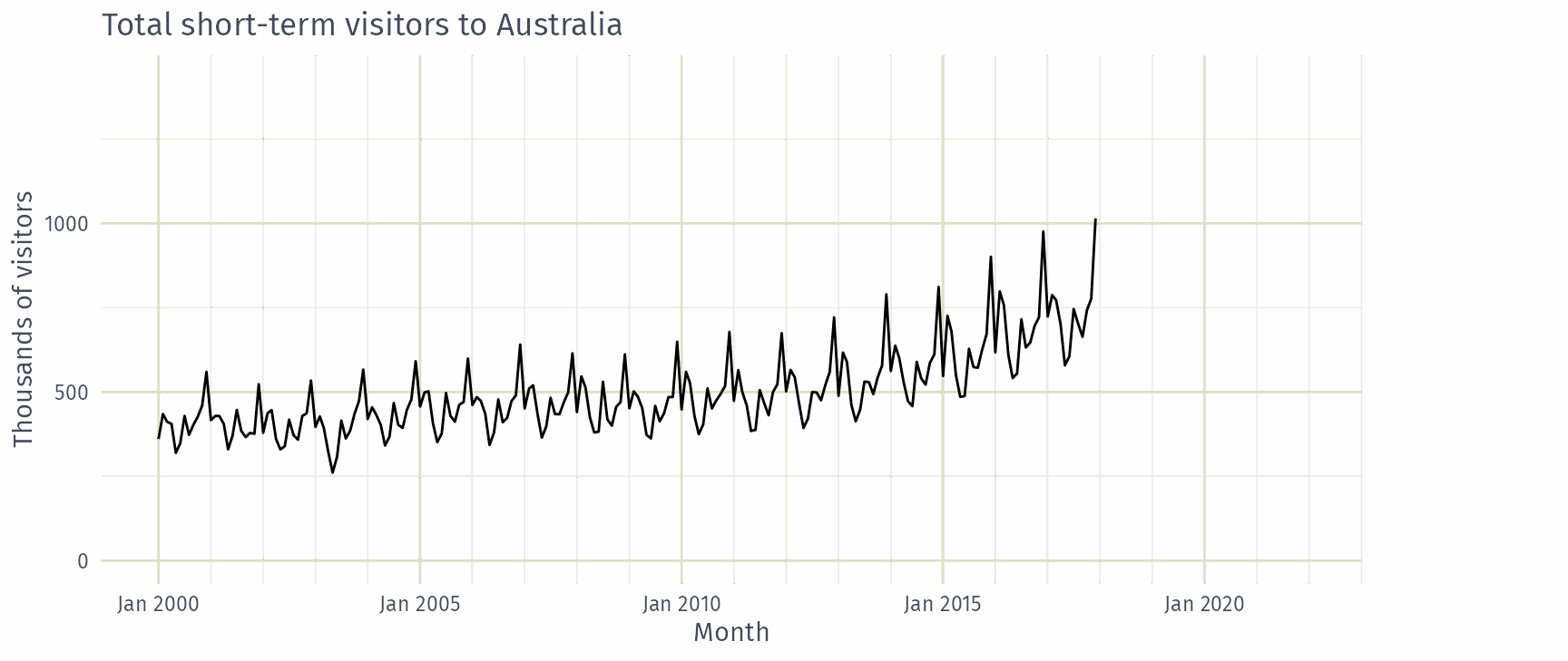
A forecast is an estimate of the probability distribution of a variable to be observed in the future.
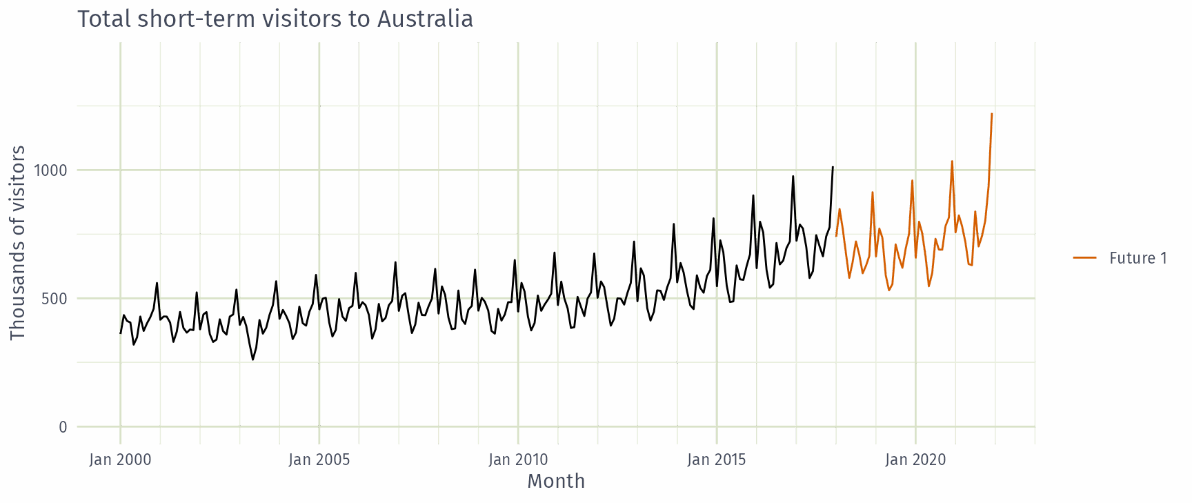
A forecast is an estimate of the probability distribution of a variable to be observed in the future.
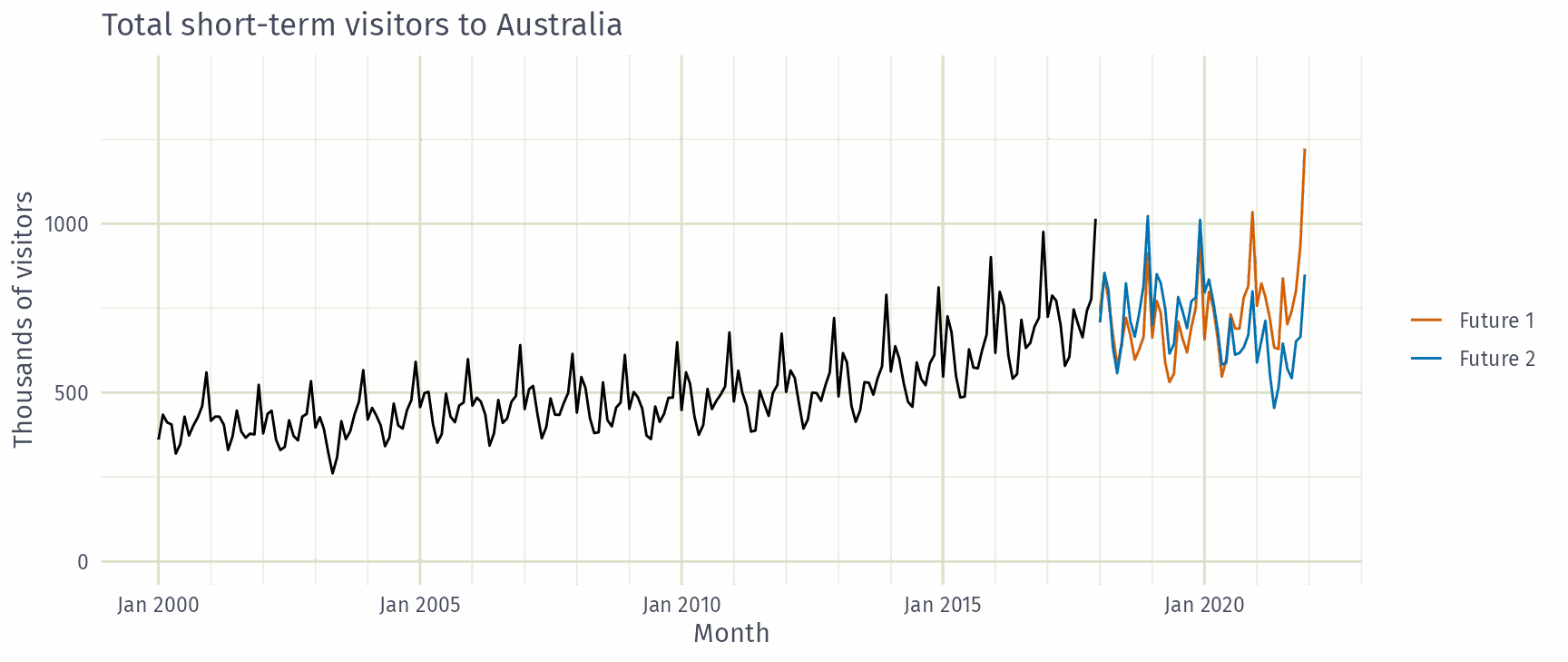
Simulated futures from an ETS model
A forecast is an estimate of the probability distribution of a variable to be observed in the future.
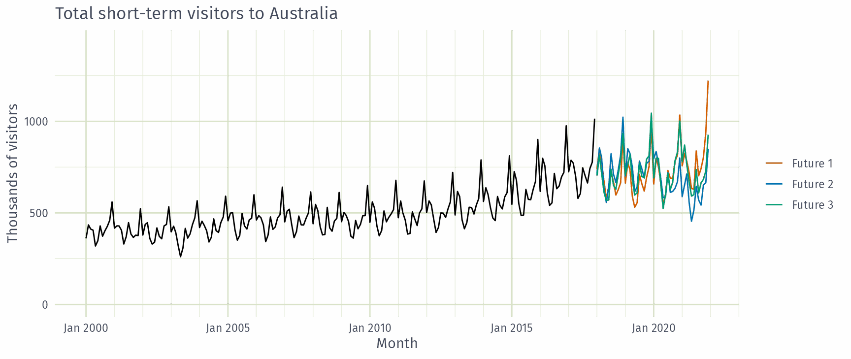
Simulated futures from an ETS model
A forecast is an estimate of the probability distribution of a variable to be observed in the future.
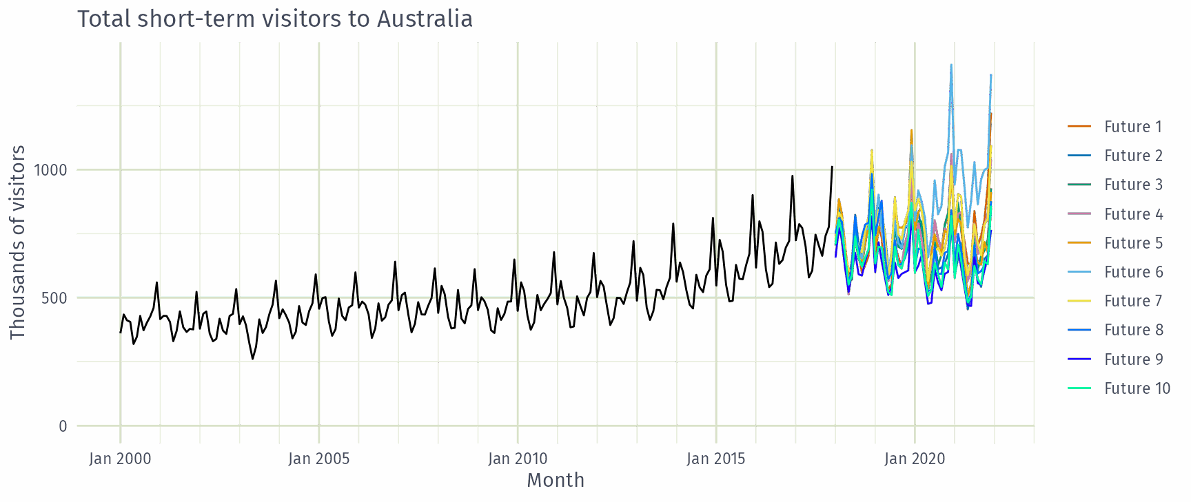
Simulated futures from an ETS model
A forecast is an estimate of the probability distribution of a variable to be observed in the future.
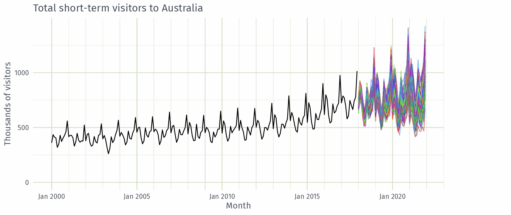
Simulated futures from an ETS model
A forecast is an estimate of the probability distribution of a variable to be observed in the future.
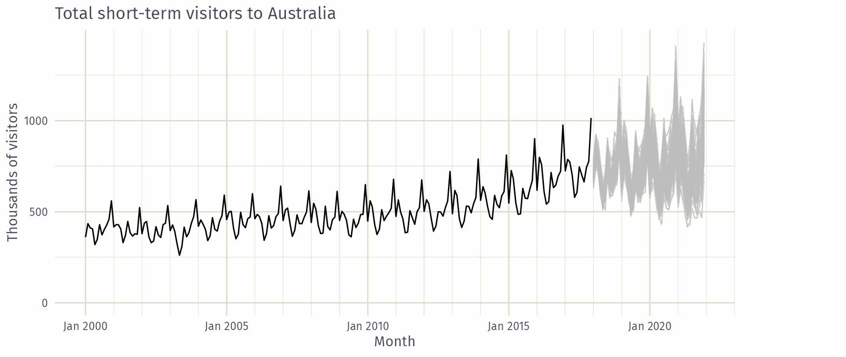
Simulated futures from an ETS model
A forecast is an estimate of the probability distribution of a variable to be observed in the future.
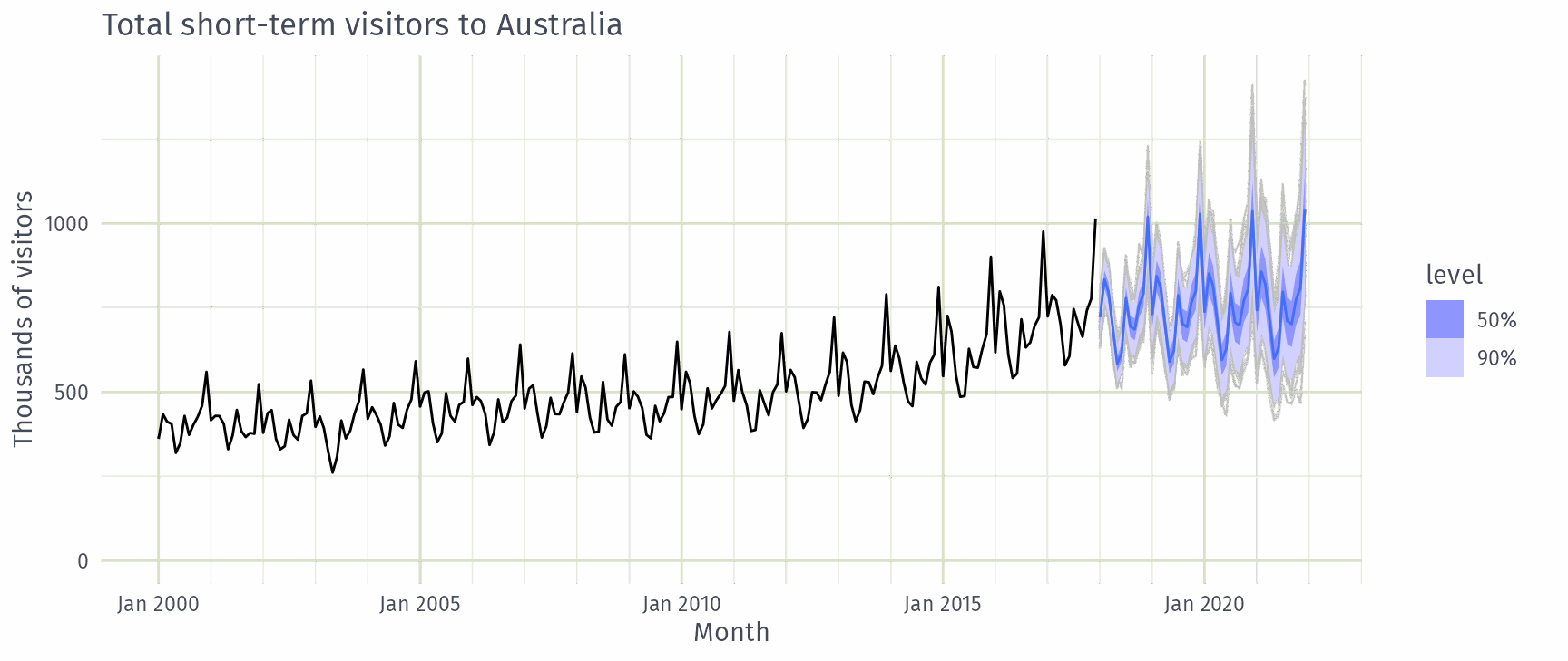
Simulated futures from an ETS model
A forecast is an estimate of the probability distribution of a variable to be observed in the future.
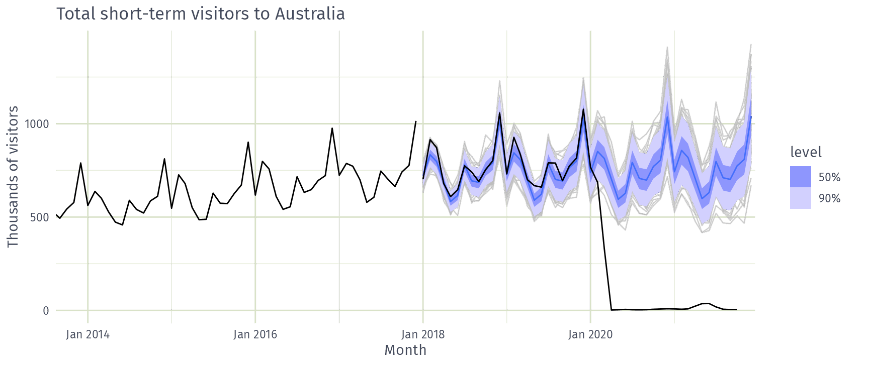
Simulated futures from an ETS model
A forecast is an estimate of the probability distribution of a variable to be observed in the future.
Simulated futures from an ETS model
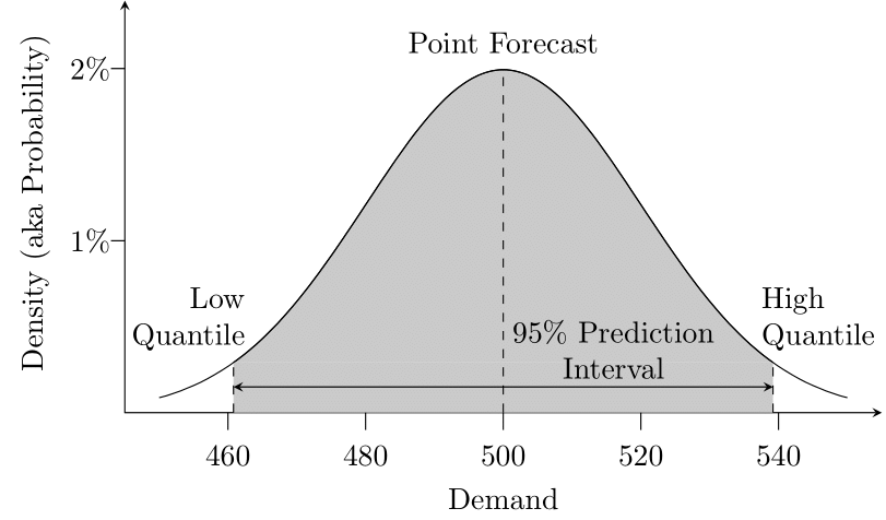
A 90% prediction interval contains the future value with 90% probability.
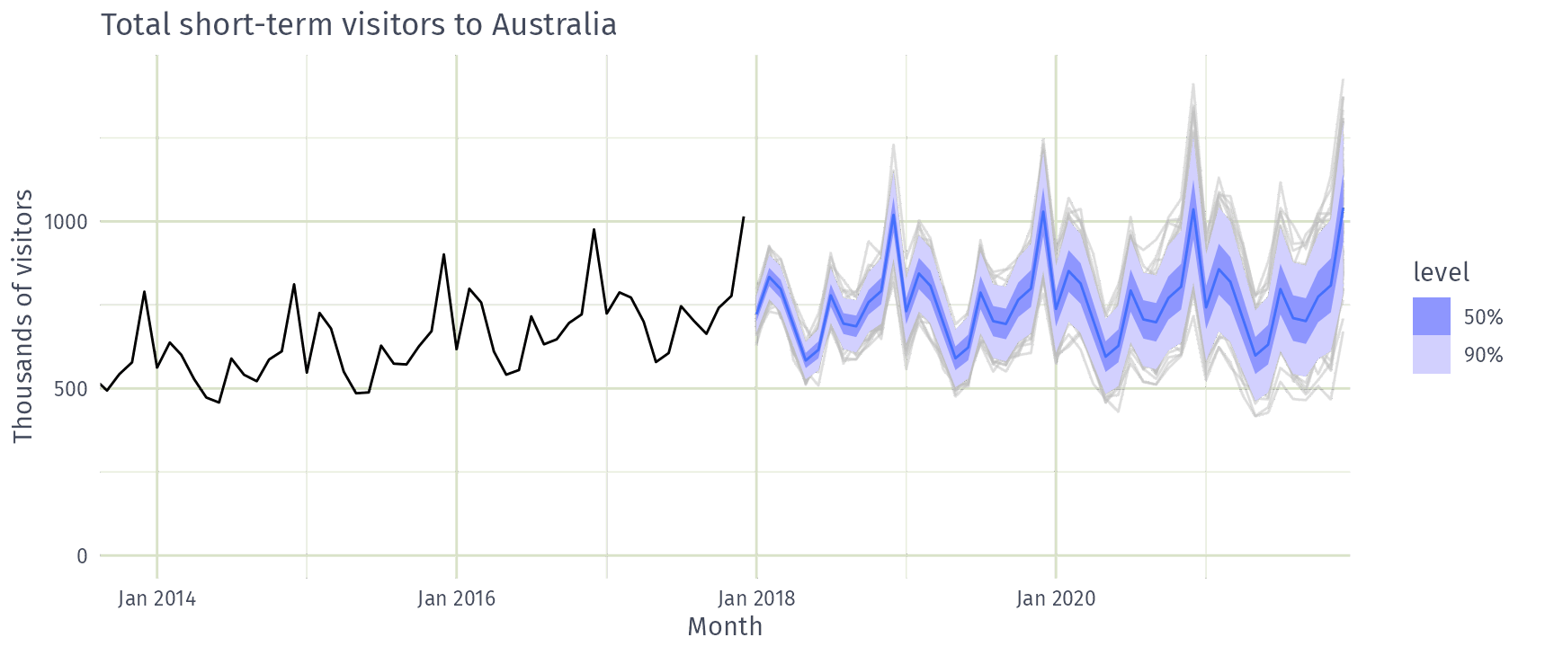
Simulated futures from an ETS model
Something is easier to forecast if:
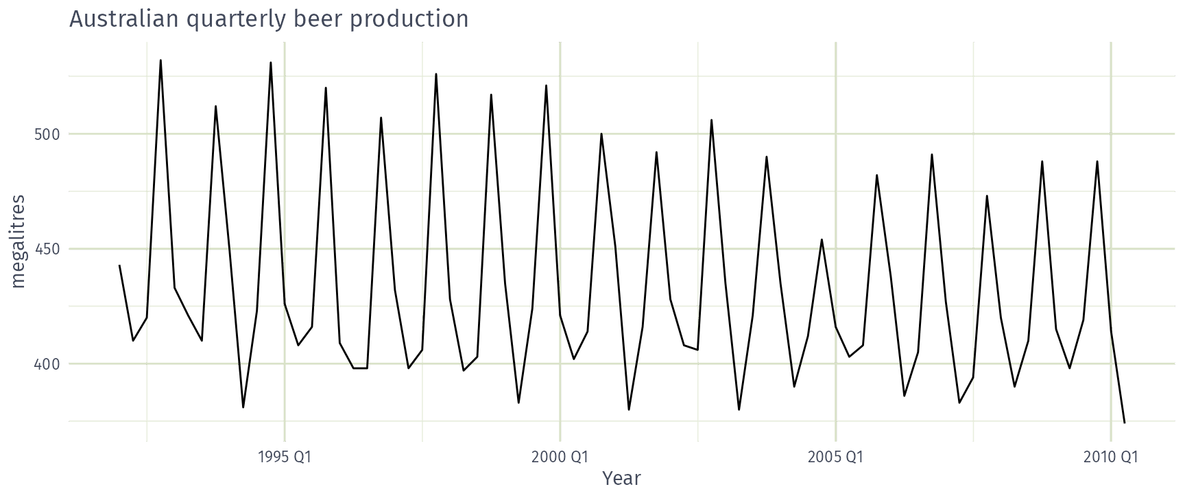
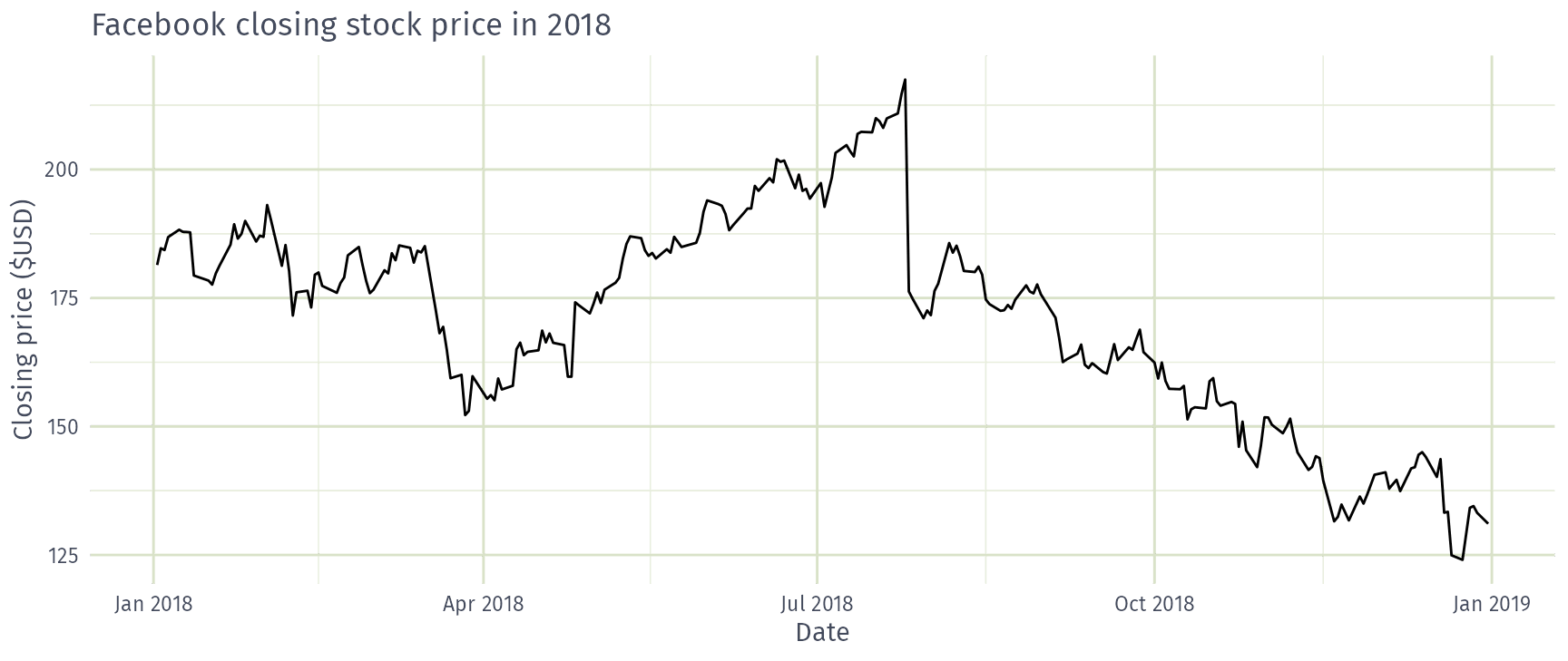
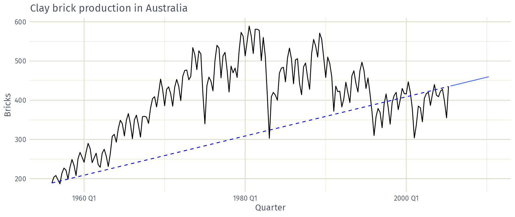
How would you forecast these series?
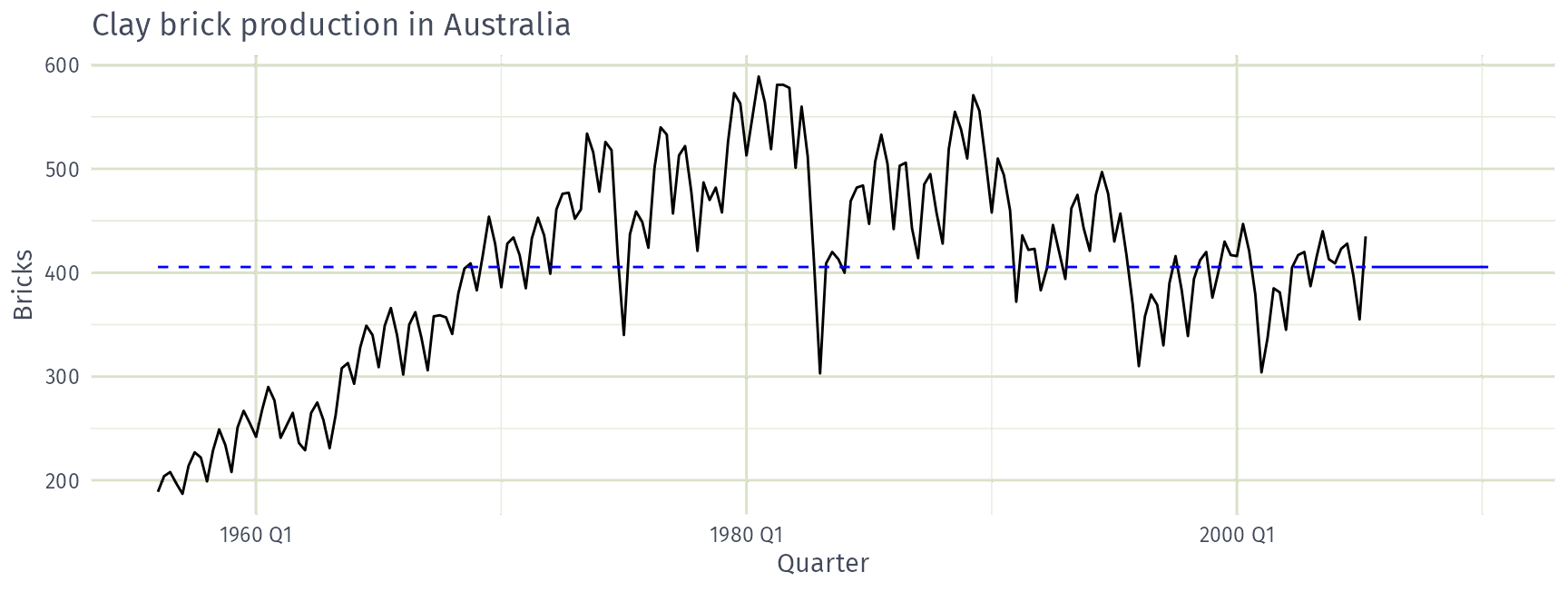
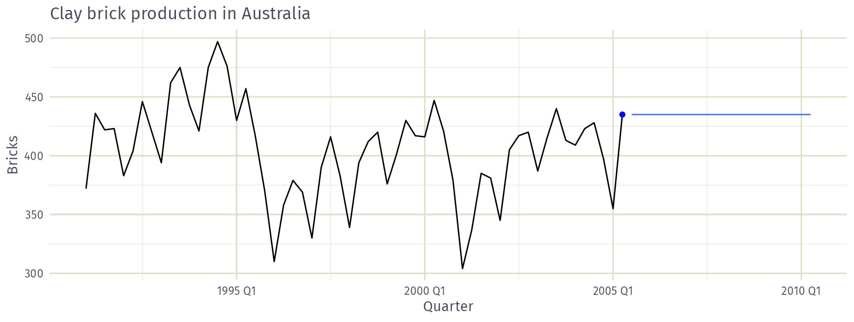
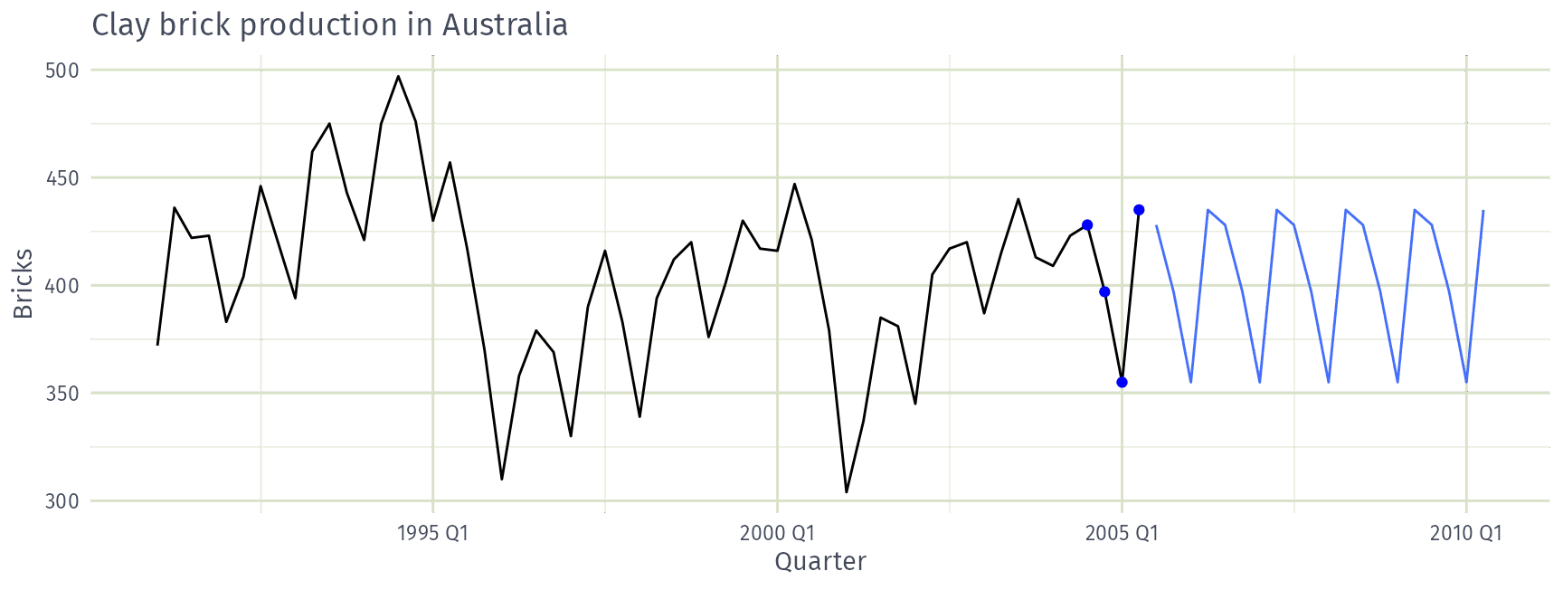
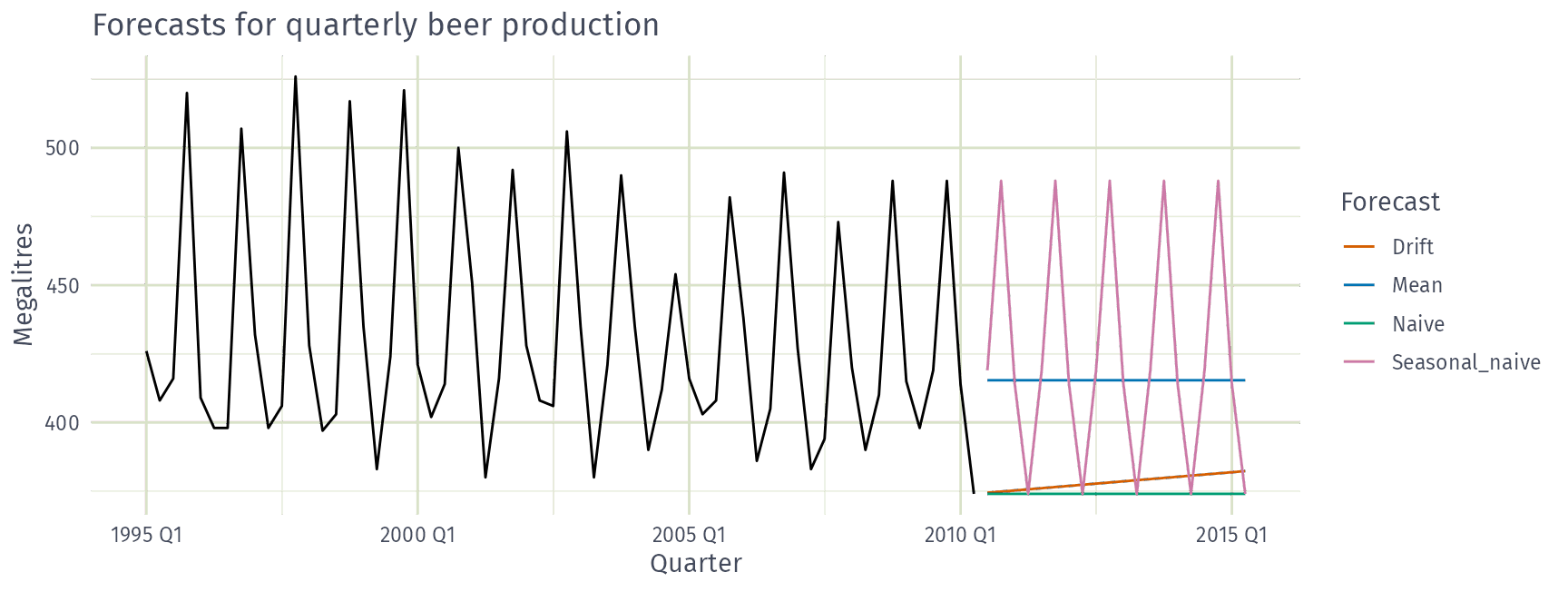
MEAN(y): Average methodNAIVE(y): Naïve methodSNAIVE(y ~ lag(m)): Seasonal naïve methodlag() defaults to the seasonal period, so SNAIVE(y) is enough.RW(y ~ drift()): Drift method\[\begin{aligned} \hat{y}_{T+h|T} & = y_{T} + \frac{h}{T-1}\sum_{t=2}^T (y_t-y_{t-1})\\ & = y_T + \frac{h}{T-1}(y_T -y_1). \end{aligned}\]
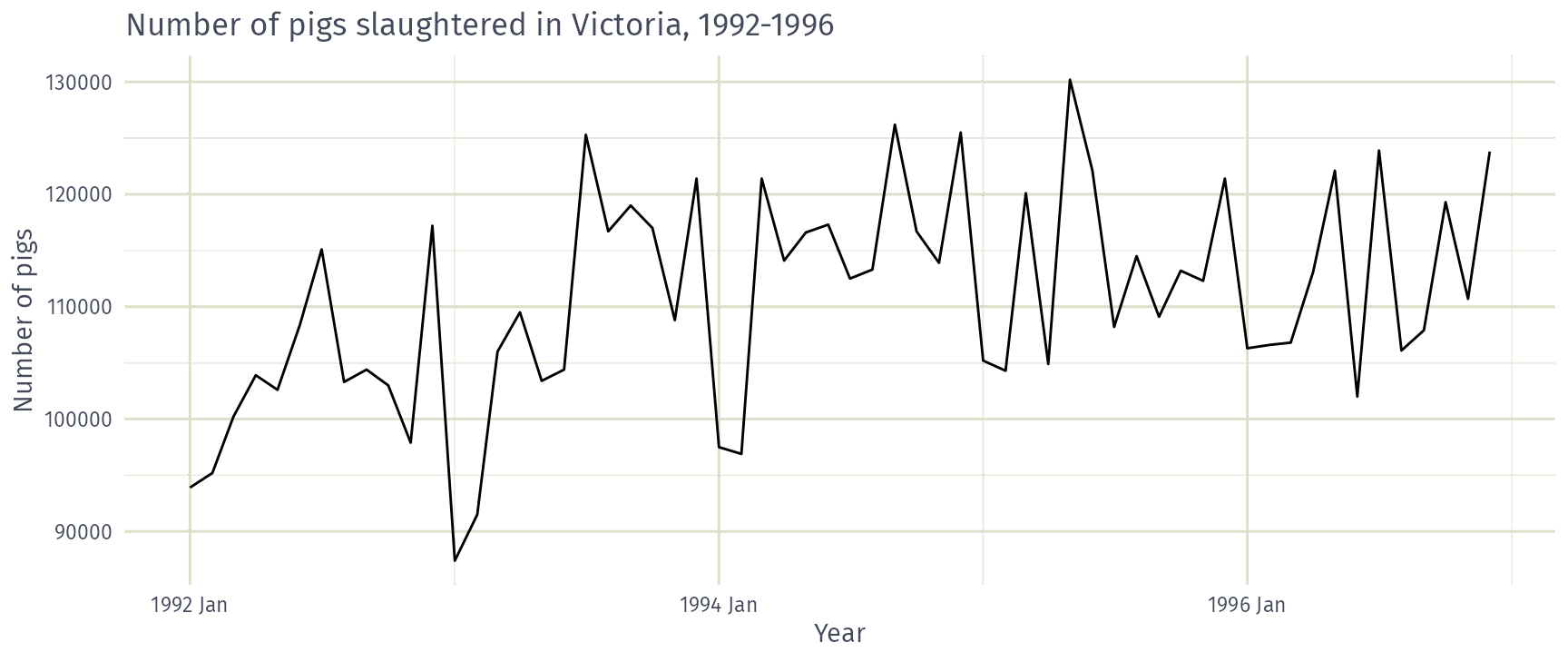
Which benchmark method is best for the number of pigs slaughtered in Victoria?
MEAN()NAIVE()SNAIVE()RW(~ drift())response ~ terms:
SNAIVE(Beer ~ lag("year")) or RW(Beer ~ drift()).The model() function trains models on data.
# A mable: 1 x 4
Seasonal_naive Naive Drift Mean
<model> <model> <model> <model>
1 <SNAIVE> <NAIVE> <RW w/ drift> <MEAN>
A mable is a model table, each cell corresponds to a fitted model.
mablereport() gives a formatted model-specific display.tidy() extracts the estimated parameters (if any) of each model.glance() gives one row of summary statistics per model, such as sigma2.select() and filter() pick out specific models.forecast() function is used to produce forecasts from estimated models.h as a number (the number of future observations);h as natural language (the length of time to predict, e.g. "5 years");new_data, a dataset of future time periods.# A fable: 80 x 4 [1Q]
# Key: .model [4]
.model Quarter Beer .mean
<chr> <qtr> <dist> <dbl>
1 Seasonal_naive 2010 Q3 N(419, 373) 419
2 Seasonal_naive 2010 Q4 N(488, 373) 488
3 Seasonal_naive 2011 Q1 N(414, 373) 414
4 Seasonal_naive 2011 Q2 N(374, 373) 374
# ℹ 76 more rows
A fable is a forecast table with point forecasts and distributions.
Assuming residuals are normal and uncorrelated, with variance \(\hat\sigma^2\):
| Mean: | \(y_{T+h|T} \sim N(\bar{y}, (1 + 1/T)\hat{\sigma}^2)\) |
| Naïve: | \(y_{T+h|T} \sim N(y_T, h\hat{\sigma}^2)\) |
| Seasonal naïve: | \(y_{T+h|T} \sim N(y_{T+h-m(k+1)}, (k+1)\hat{\sigma}^2)\) |
| Drift: | \(y_{T+h|T} \sim N(y_T + \frac{h}{T-1}(y_T - y_1),h\frac{T+h}{T}\hat{\sigma}^2)\) |
where \(k\) is the integer part of \((h-1)/m\).
Note that when \(h=1\) and \(T\) is large, these all give the same approximate forecast variance: \(\hat{\sigma}^2\).
When a normal distribution for the residuals is an unreasonable assumption, one alternative is to use bootstrapping, which only assumes that the residuals are uncorrelated with constant variance.
A residual (one-step forecast error) is \(e_t = y_t - \hat{y}_{t|t-1}\), so \(y_t = \hat{y}_{t|t-1} + e_t\).
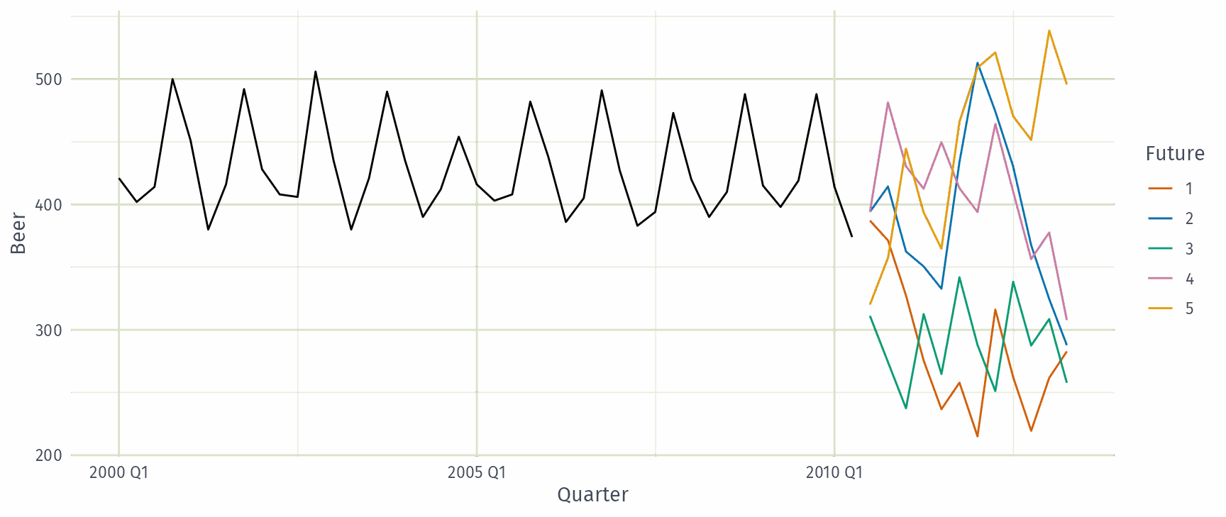
So we can simulate the next observation of a time series using \(y_{T+1} = \hat{y}_{T+1|T} + e_{T+1}\), where \(e_{T+1}\) is sampled (with replacement) from the past residuals.
Adding the new simulated observation to our data set, we can repeat the process to obtain \(y_{T+2} = \hat{y}_{T+2|T+1} + e_{T+2}\)
generate()# A tsibble: 60 x 4 [1Q]
# Key: .model, .rep [5]
.model Quarter .rep .sim
<chr> <qtr> <chr> <dbl>
1 NAIVE(Beer) 2010 Q3 1 387.
2 NAIVE(Beer) 2010 Q4 1 371.
3 NAIVE(Beer) 2011 Q1 1 327.
4 NAIVE(Beer) 2011 Q2 1 276.
5 NAIVE(Beer) 2011 Q3 1 237.
# ℹ 55 more rows
forecast() to produce probabilistic forecasts# A fable: 12 x 4 [1Q]
# Key: .model [1]
.model Quarter Beer .mean
<chr> <qtr> <dist> <dbl>
1 NAIVE(Beer) 2010 Q3 sample[5000] 374.
2 NAIVE(Beer) 2010 Q4 sample[5000] 375.
3 NAIVE(Beer) 2011 Q1 sample[5000] 375.
4 NAIVE(Beer) 2011 Q2 sample[5000] 374.
5 NAIVE(Beer) 2011 Q3 sample[5000] 374.
6 NAIVE(Beer) 2011 Q4 sample[5000] 374.
7 NAIVE(Beer) 2012 Q1 sample[5000] 375.
8 NAIVE(Beer) 2012 Q2 sample[5000] 374.
9 NAIVE(Beer) 2012 Q3 sample[5000] 376.
10 NAIVE(Beer) 2012 Q4 sample[5000] 376.
11 NAIVE(Beer) 2013 Q1 sample[5000] 375.
12 NAIVE(Beer) 2013 Q2 sample[5000] 375.
hilo() function.# A tsibble: 8 x 3 [1Q]
Quarter .mean `95%`
<qtr> <dbl> <hilo>
1 2010 Q3 374 [241.36, 507]95
2 2010 Q4 374 [186.42, 562]95
3 2011 Q1 374 [144.27, 604]95
4 2011 Q2 374 [108.73, 639]95
5 2011 Q3 374 [ 77.42, 671]95
6 2011 Q4 374 [ 49.11, 699]95
7 2012 Q1 374 [ 23.08, 725]95
8 2012 Q2 374 [ -1.15, 749]95
# A tsibble: 20 x 4 [1Q]
Quarter .mean `50%` `75%`
<qtr> <dbl> <hilo> <hilo>
1 2010 Q3 419 [406, 432]50 [397, 441]75
2 2010 Q4 488 [475, 501]50 [466, 510]75
3 2011 Q1 414 [401, 427]50 [392, 436]75
4 2011 Q2 374 [361, 387]50 [352, 396]75
5 2011 Q3 419 [401, 437]50 [388, 450]75
6 2011 Q4 488 [470, 506]50 [457, 519]75
7 2012 Q1 414 [396, 432]50 [383, 445]75
8 2012 Q2 374 [356, 392]50 [343, 405]75
9 2012 Q3 419 [396, 442]50 [380, 458]75
10 2012 Q4 488 [465, 511]50 [449, 527]75
11 2013 Q1 414 [391, 437]50 [375, 453]75
12 2013 Q2 374 [351, 397]50 [335, 413]75
13 2013 Q3 419 [393, 445]50 [375, 463]75
14 2013 Q4 488 [462, 514]50 [444, 532]75
15 2014 Q1 414 [388, 440]50 [370, 458]75
16 2014 Q2 374 [348, 400]50 [330, 418]75
17 2014 Q3 419 [390, 448]50 [369, 469]75
18 2014 Q4 488 [459, 517]50 [438, 538]75
19 2015 Q1 414 [385, 443]50 [364, 464]75
20 2015 Q2 374 [345, 403]50 [324, 424]75
# A tsibble: 20 x 3 [1Q]
Quarter `50%_lower` `50%_upper`
<qtr> <dbl> <dbl>
1 2010 Q3 406. 432.
2 2010 Q4 475. 501.
3 2011 Q1 401. 427.
4 2011 Q2 361. 387.
5 2011 Q3 401. 437.
6 2011 Q4 470. 506.
7 2012 Q1 396. 432.
8 2012 Q2 356. 392.
9 2012 Q3 396. 442.
10 2012 Q4 465. 511.
11 2013 Q1 391. 437.
12 2013 Q2 351. 397.
13 2013 Q3 393. 445.
14 2013 Q4 462. 514.
15 2014 Q1 388. 440.
16 2014 Q2 348. 400.
17 2014 Q3 390. 448.
18 2014 Q4 459. 517.
19 2015 Q1 385. 443.
20 2015 Q2 345. 403.
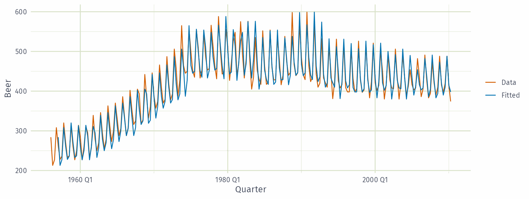
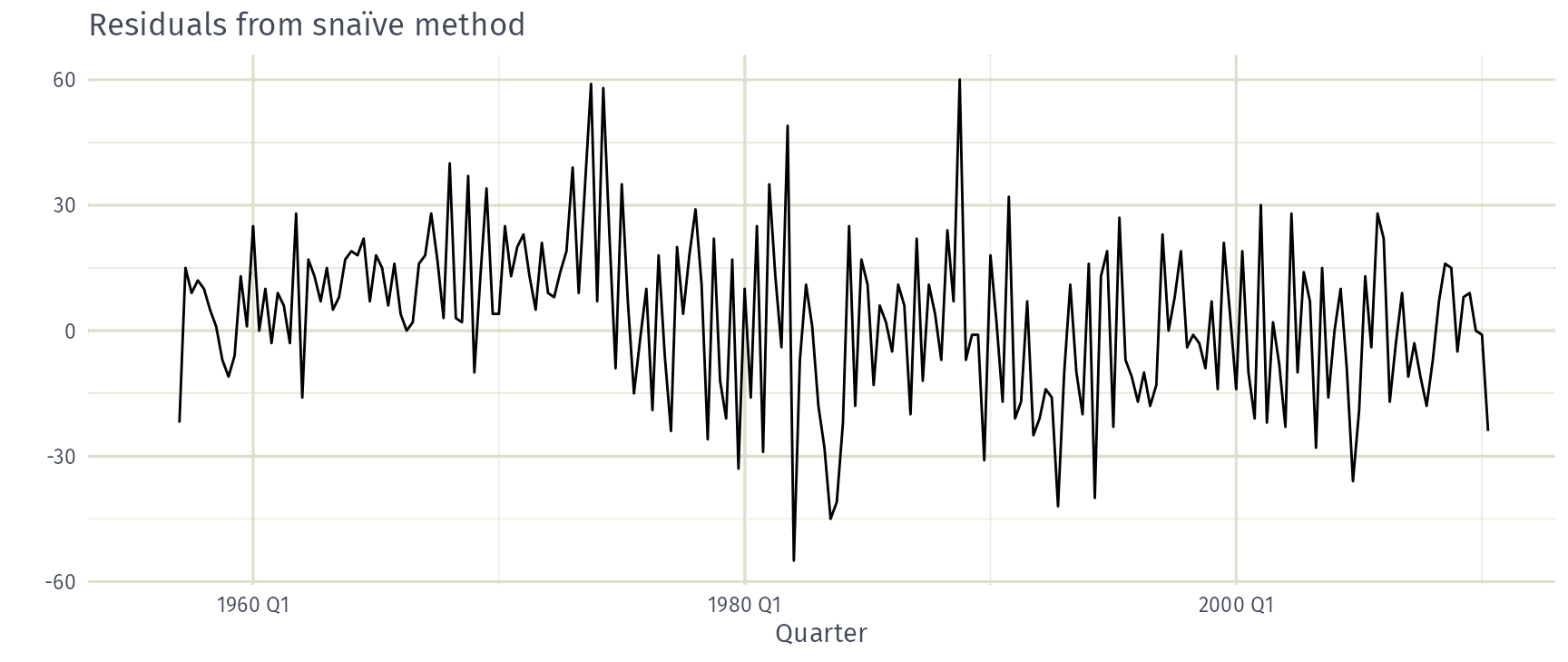
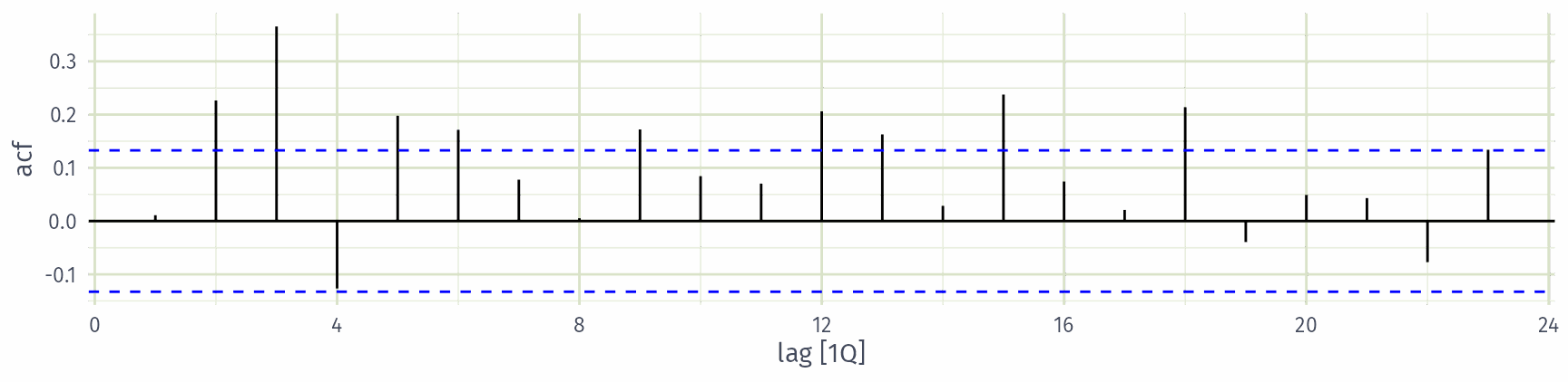
Residuals in forecasting: difference between observed value and its fitted value: \(e_t = y_t-\hat{y}_{t|t-1}\).
augment() gives both .resid and .innov (innovation residuals); they are equal unless the response is transformed.# A tsibble: 218 x 6 [1Q]
# Key: .model [1]
.model Quarter Beer .fitted .resid .innov
<chr> <qtr> <dbl> <dbl> <dbl> <dbl>
1 SNAIVE(Beer) 1956 Q1 284 NA NA NA
2 SNAIVE(Beer) 1956 Q2 213 NA NA NA
3 SNAIVE(Beer) 1956 Q3 227 NA NA NA
4 SNAIVE(Beer) 1956 Q4 308 NA NA NA
5 SNAIVE(Beer) 1957 Q1 262 284 -22 -22
6 SNAIVE(Beer) 1957 Q2 228 213 15 15
7 SNAIVE(Beer) 1957 Q3 236 227 9 9
8 SNAIVE(Beer) 1957 Q4 320 308 12 12
9 SNAIVE(Beer) 1958 Q1 272 262 10 10
10 SNAIVE(Beer) 1958 Q2 233 228 5 5
# ℹ 208 more rows
These residuals look like random noise
Scale: Strongly disagree · Disagree · Neutral · Agree · Strongly agree