AFRICAST

Tidy time series & forecasting in R

Time series patterns and basic graphics

Session 2 of 10

workshop.f4sg.org/africastForecasting for Social Good

Time series Patterns

Key patterns of time series

• Level

• Underlying trend

• Seasonal/cycle

• Autocorrelation

• Unpredictable patterns/Noise

• Different types of events and driving factors (i.e. predictors) may affect the time series

Time series patterns

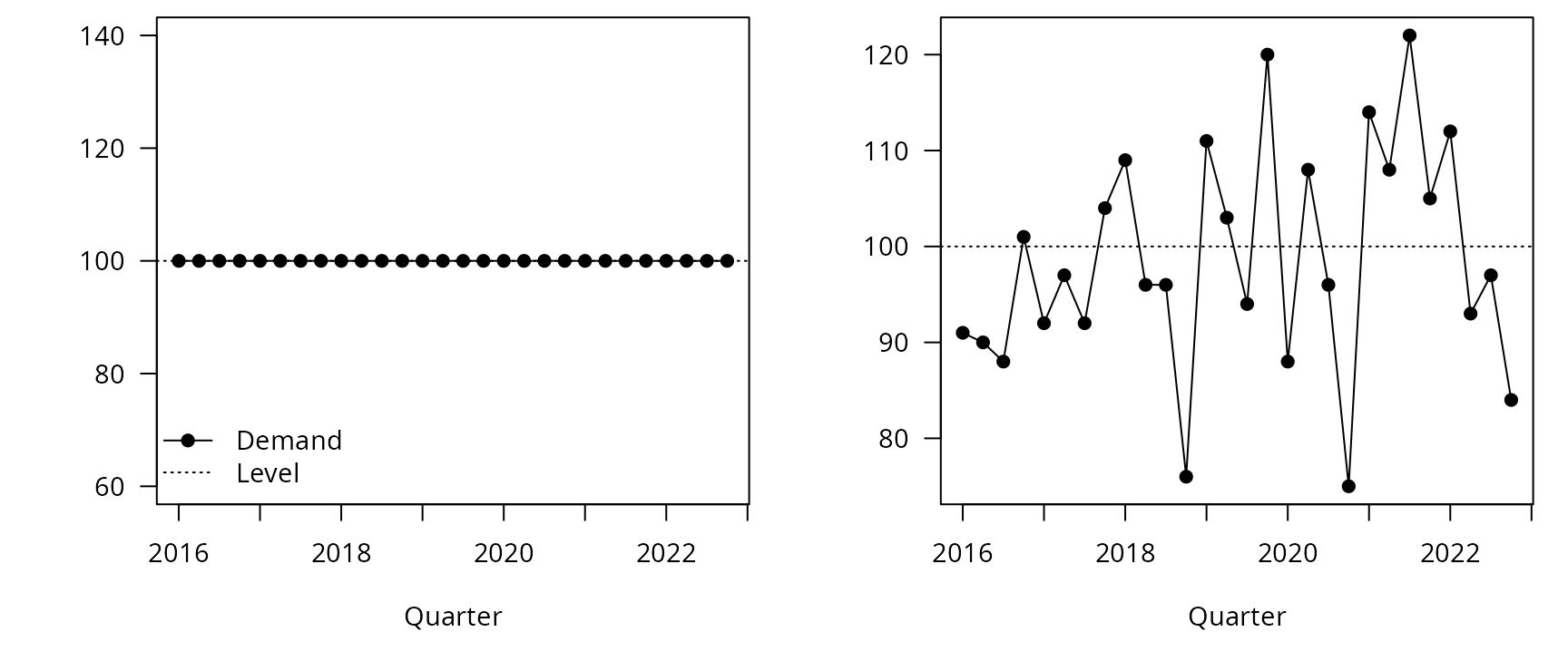
Level

The level of a time series describes the centre of the series.

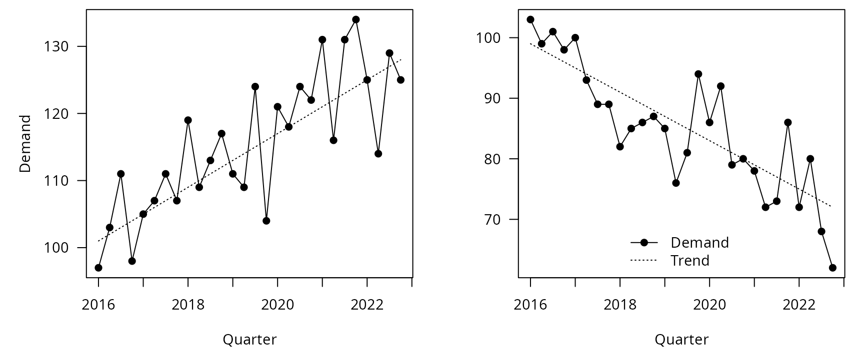
Trend

A trend describes predictable increases or decreases in the level of a series.

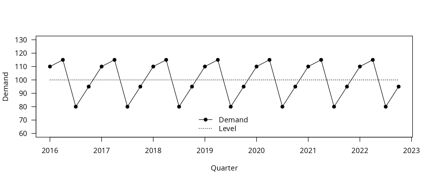
Seasonal

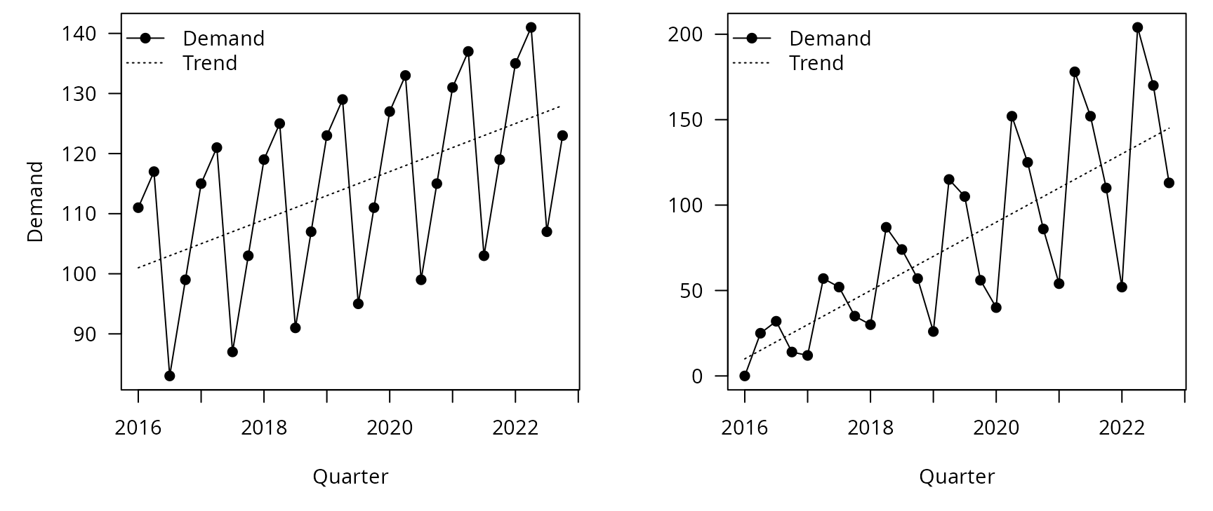
Seasonality is a consistent pattern that repeats over a fixed period of time. pattern exists when a series is influenced by seasonal factors (e.g., the quarter of the year, the month, or day of the week).

Cyclic

pattern exists when data exhibit rises and falls that are not of fixed period (duration usually of at least 2 years).

Level

Trend

Seasonality

Additive versus multiplicative seasonality

Cycles

Time plots

Time plots

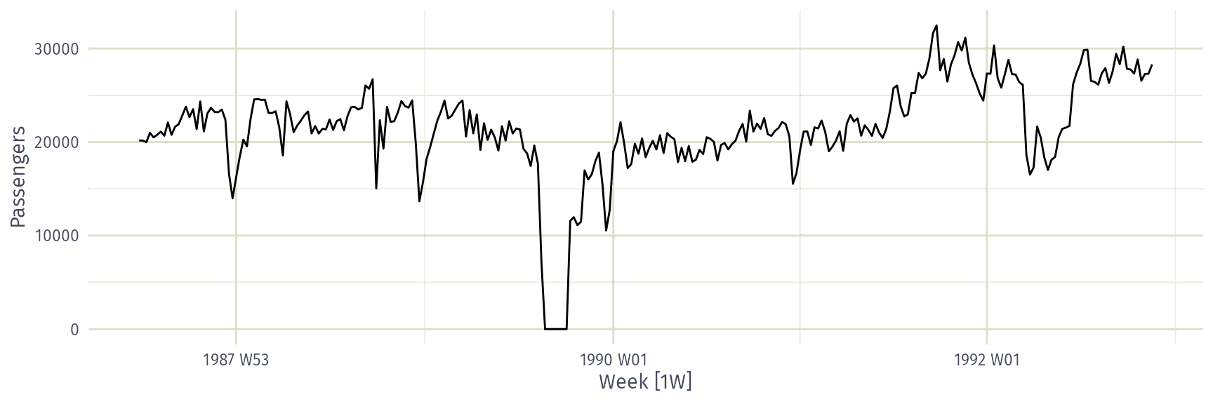
ansett |>
  filter(Airports=="MEL-SYD", Class=="Economy") |>
  autoplot(Passengers)

Time plots

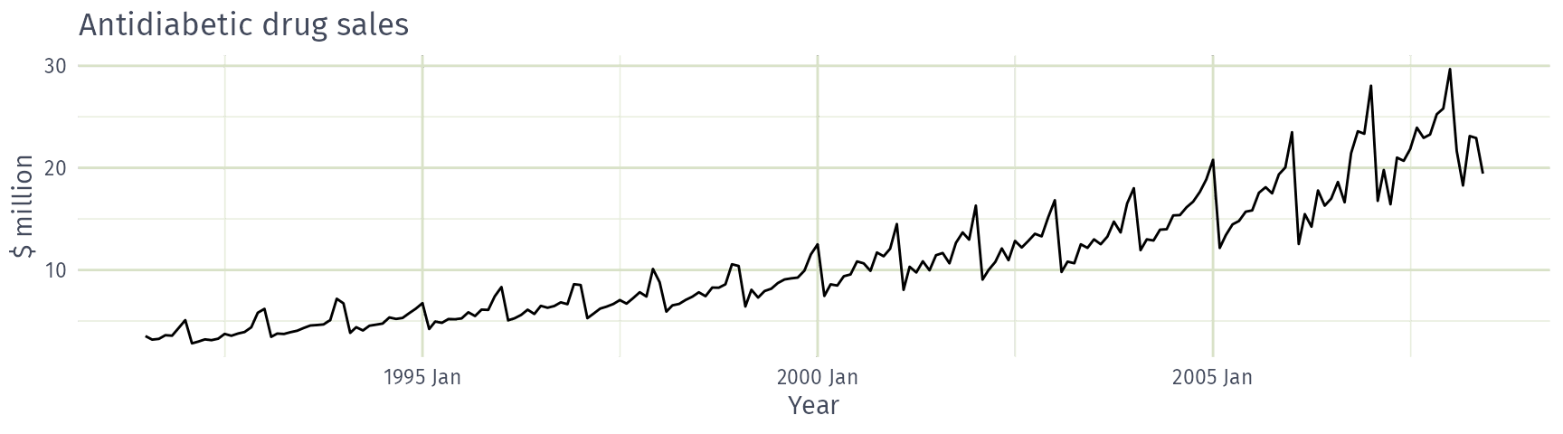
PBS |> filter(ATC2 == "A10") |>
  summarise(Cost = sum(Cost)/1e6) |> autoplot(Cost) +
  labs(x = "Year", y = "$ million", title = "Antidiabetic drug sales")

Seasonal plots

Seasonal plots

• Data plotted against the individual “seasons” in which the data were observed. (In this case a “season” is a month.)
• Something like a time plot except that the data from each season are overlapped.
• Enables the underlying seasonal pattern to be seen more clearly, and also allows any substantial departures from the seasonal pattern to be easily identified.
• In R: gg_season() (ggtime)

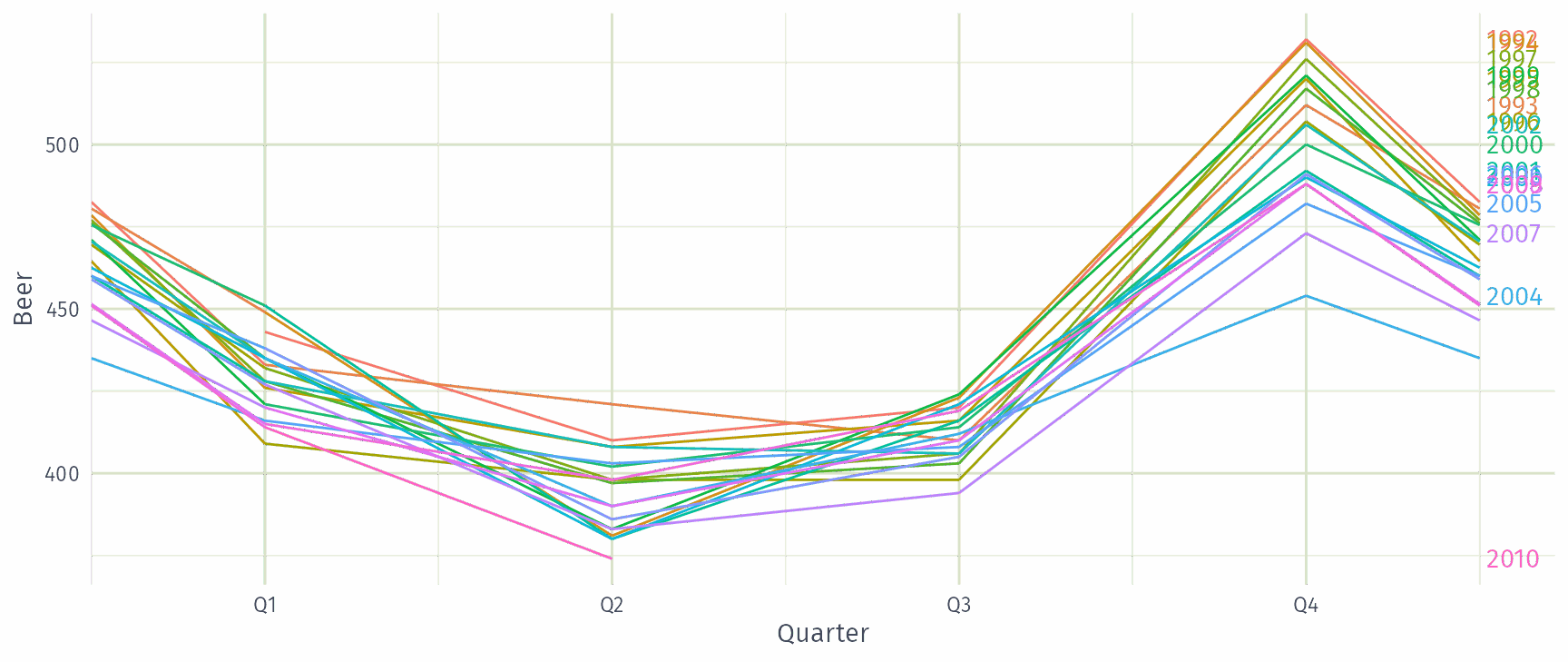
Building a seasonal plot

Time plot of quarterly Australian beer production since 1992.

Each observation belongs to a year. Split the line between years, half-way between Q4 and the next Q1.

Move each year back to the start in turn, stacking them. The time axis narrows to a single year.

Remove the points: the seasonal plot, with one line per year.

Quarterly Australian Beer Production

beer |> gg_season(Beer, labels = "right")

Multiple seasonal periods

vic_elec

# A tsibble: 52,608 x 5 [30m] <Australia/Melbourne>
   Time                Demand Temperature Date       Holiday
   <dttm>               <dbl>       <dbl> <date>     <lgl>  
 1 2012-01-01 00:00:00  4383.        21.4 2012-01-01 TRUE   
 2 2012-01-01 00:30:00  4263.        21.0 2012-01-01 TRUE   
 3 2012-01-01 01:00:00  4049.        20.7 2012-01-01 TRUE   
 4 2012-01-01 01:30:00  3878.        20.6 2012-01-01 TRUE   
 5 2012-01-01 02:00:00  4036.        20.4 2012-01-01 TRUE   
 6 2012-01-01 02:30:00  3866.        20.2 2012-01-01 TRUE   
 7 2012-01-01 03:00:00  3694.        20.1 2012-01-01 TRUE   
 8 2012-01-01 03:30:00  3562.        19.6 2012-01-01 TRUE   
 9 2012-01-01 04:00:00  3433.        19.1 2012-01-01 TRUE   
10 2012-01-01 04:30:00  3359.        19.0 2012-01-01 TRUE   
# ℹ 52,598 more rows

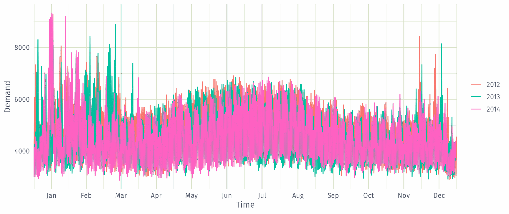
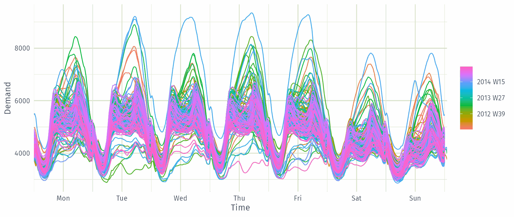
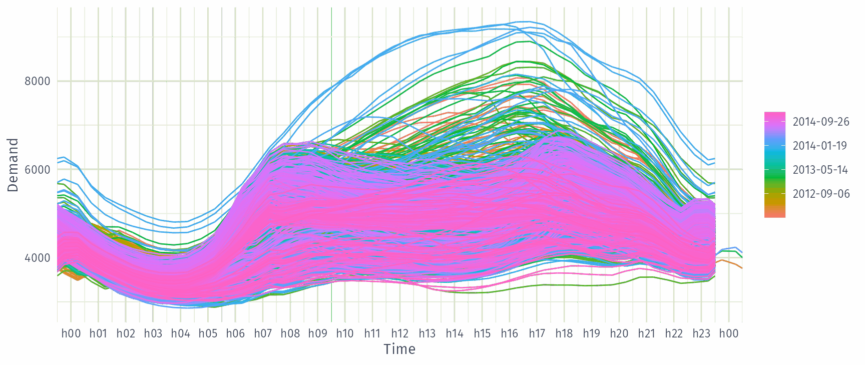
Multiple seasonal periods

vic_elec |> gg_season(Demand)

Multiple seasonal periods

vic_elec |> gg_season(Demand, period = "week")

Multiple seasonal periods

vic_elec |> gg_season(Demand, period = "day")

Seasonal subseries plots

• Data for each season collected together in time plot as separate time series.
• Enables the underlying seasonal pattern to be seen clearly, and changes in seasonality over time to be visualised.
• In R: gg_subseries() (ggtime)

Building a seasonal subseries plot

Time plot of quarterly Australian beer production since 1992.

Each observation belongs to a quarter of the year.

Join the observations from the same quarter: four subseries, each a time series in its own right.

Separate the subseries and place them side by side to compare the quarters.

Add the mean of each quarter: the seasonal subseries plot.

Australian holidays

holidays <- tourism |>
  filter(Purpose == "Holiday") |>
  group_by(State) |>
  summarise(Trips = sum(Trips))

# A tsibble: 640 x 3 [1Q]
# Key:       State [8]
   State Quarter Trips
   <chr>   <qtr> <dbl>
 1 ACT   1998 Q1  196.
 2 ACT   1998 Q2  127.
 3 ACT   1998 Q3  111.
 4 ACT   1998 Q4  170.
 5 ACT   1999 Q1  108.
 6 ACT   1999 Q2  125.
 7 ACT   1999 Q3  178.
 8 ACT   1999 Q4  218.
 9 ACT   2000 Q1  158.
10 ACT   2000 Q2  155.
# ℹ 630 more rows

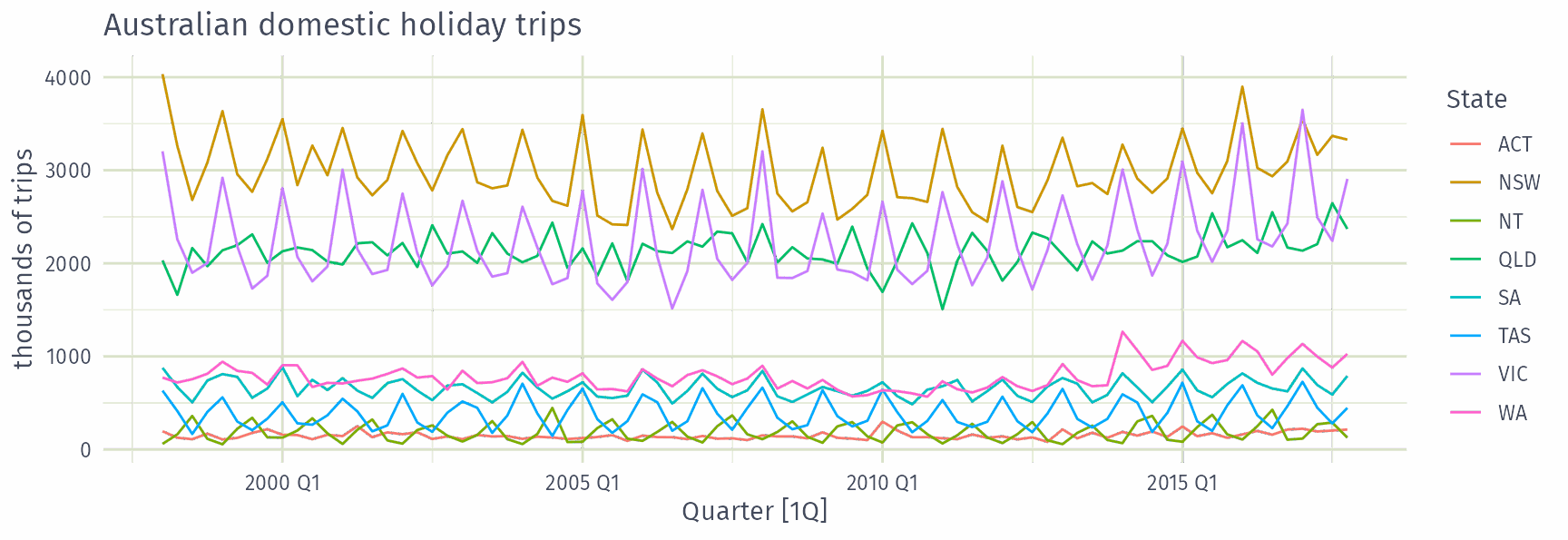
Australian holidays

holidays |> autoplot(Trips) +
  labs(y = "thousands of trips", title = "Australian domestic holiday trips")

Seasonal plots

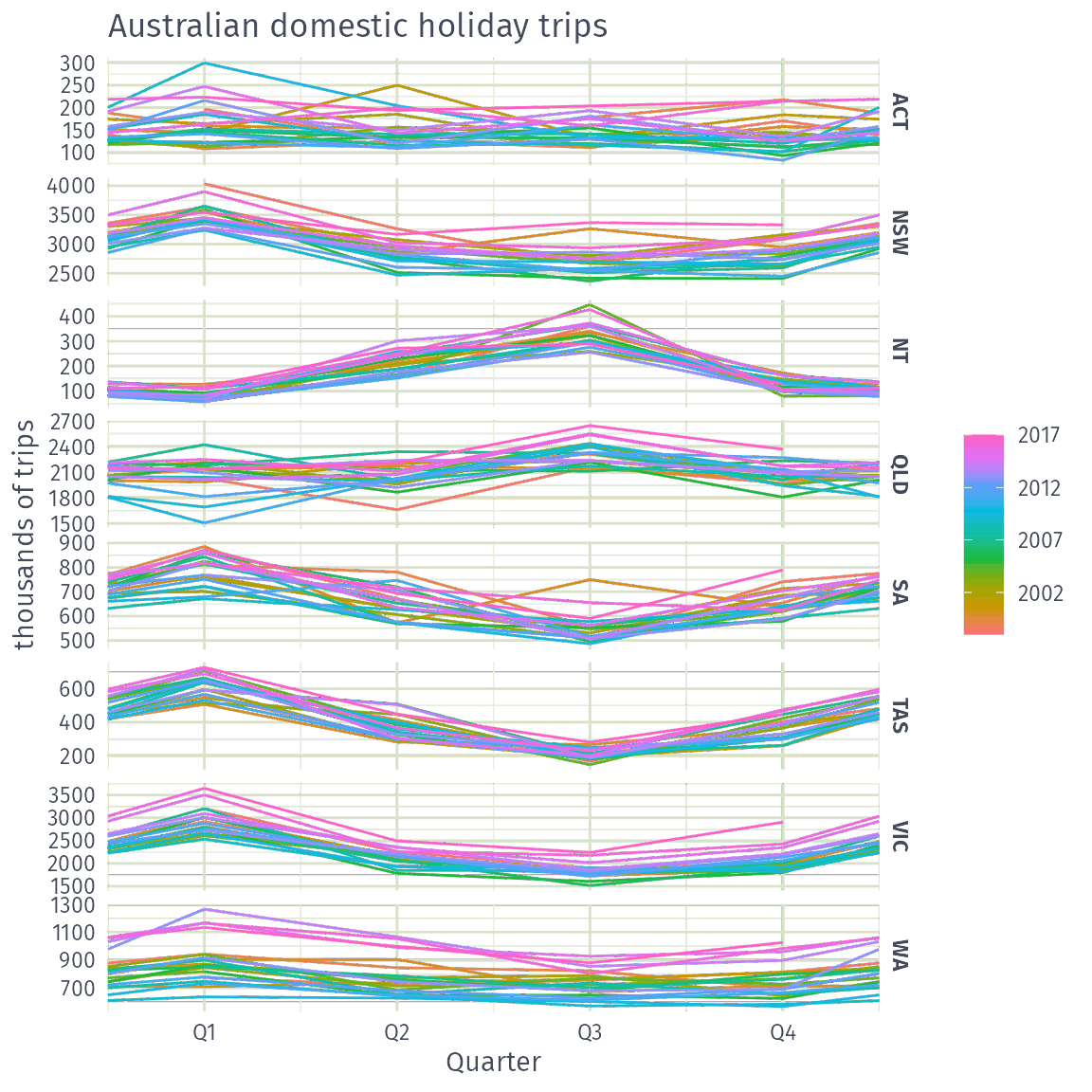
holidays |> gg_season(Trips) +
  labs(y = "thousands of trips", title = "Australian domestic holiday trips")

Seasonal subseries plots

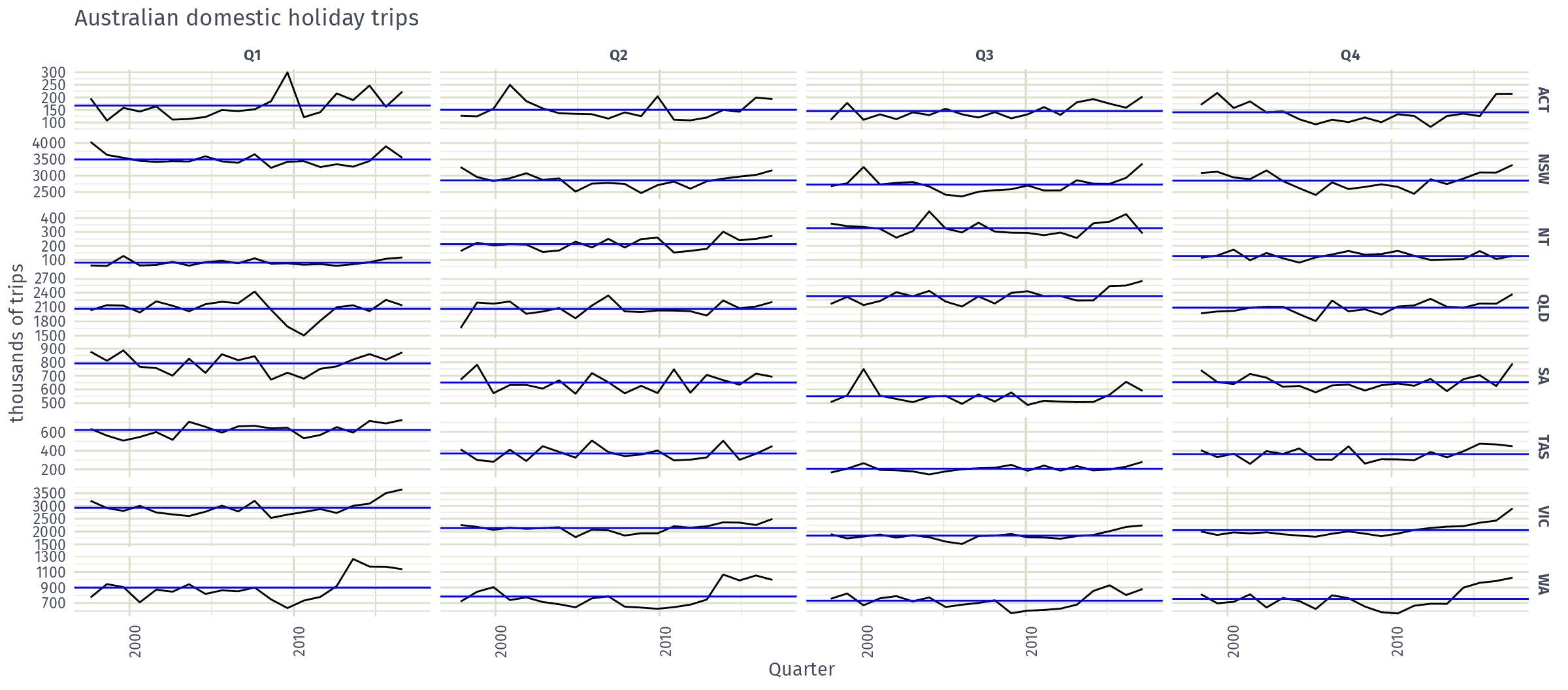
holidays |> gg_subseries(Trips) +
  labs(y = "thousands of trips", title = "Australian domestic holiday trips")

Calendar plots

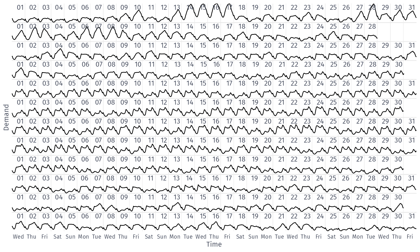
library(ggtime)
vic_elec |>
  filter(year(Date) == 2014) |>
  as_tibble() |>
  ggplot(aes(x = Time, y = Demand)) +
  geom_line() +
  coord_calendar(rows = month(1L), cols = NULL) +
  scale_x_mixtime(
    time_breaks = mixtime::days(1L),
    time_labels = "{cyc(day, cal_isoweek$week, label = TRUE, abbreviate = TRUE)}"
  ) +
  theme(axis.text.y = element_blank(), axis.ticks.y = element_blank())

• coord_calendar() cuts a time axis into a calendar-like grid of rows/columns
• each row above is a month, and each cell within it a day

Calendar plots

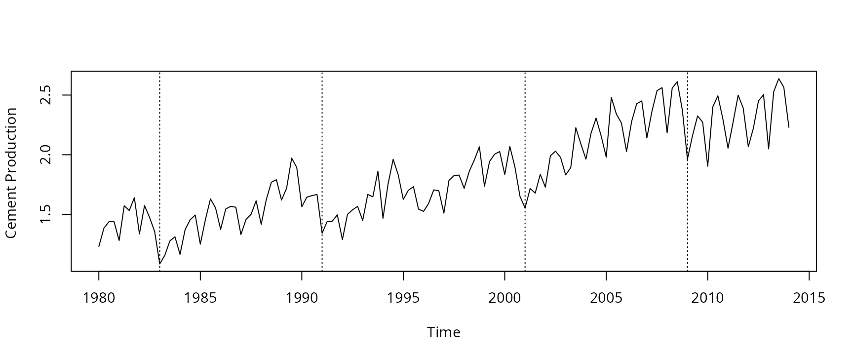
Seasonal or cyclic?

Time series patterns

Trend

pattern exists when there is a long-term increase or decrease in the data.

Seasonal

pattern exists when a series is influenced by seasonal factors (e.g., the quarter of the year, the month, or day of the week).

Cyclic

pattern exists when data exhibit rises and falls that are not of fixed period (duration usually of at least 2 years).

Time series components

Differences between seasonal and cyclic patterns:

• seasonal pattern constant length; cyclic pattern variable length
• average length of cycle longer than length of seasonal pattern
• magnitude of cycle more variable than magnitude of seasonal pattern

Time series patterns

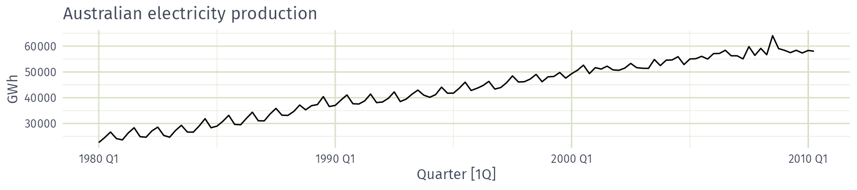
Australian electricity production: seasonal, cyclic, both or neither?

• Seasonal
• Cyclic
• Both
• Neither

Time series patterns

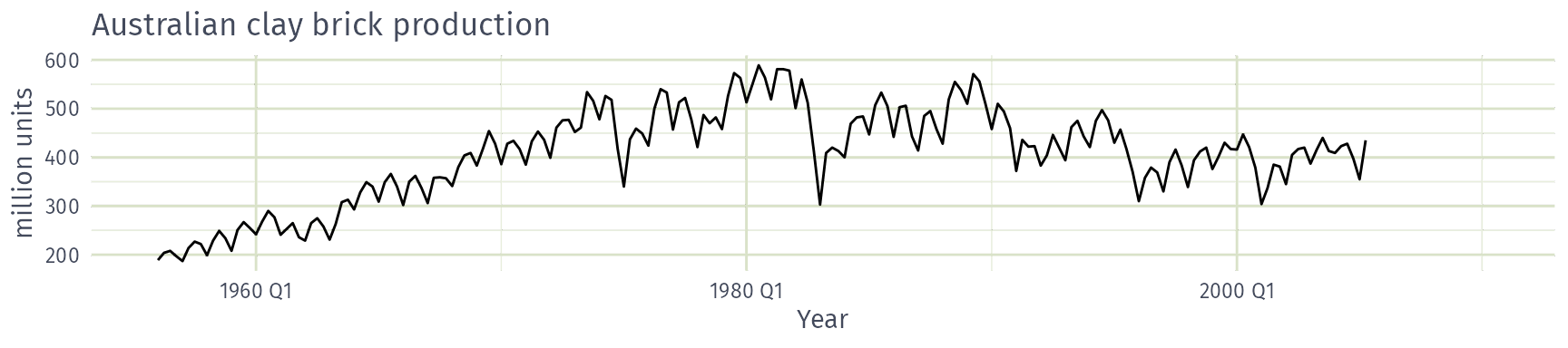
Australian clay brick production: seasonal, cyclic, both or neither?

• Seasonal
• Cyclic
• Both
• Neither

Time series patterns

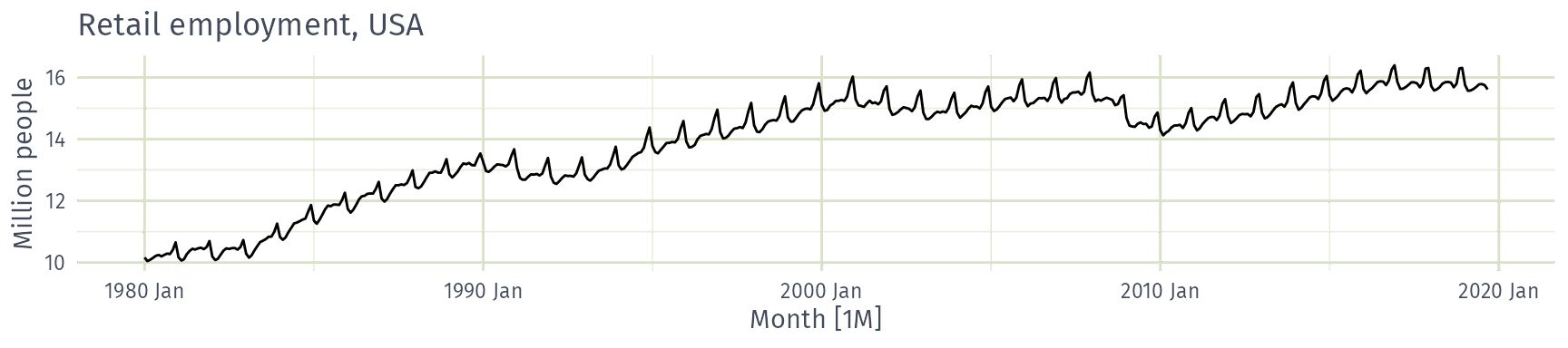
US retail employment: seasonal, cyclic, both or neither?

• Seasonal
• Cyclic
• Both
• Neither

Time series patterns

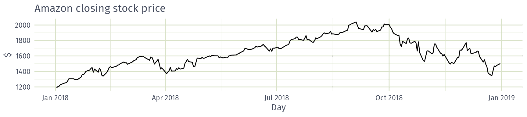
Amazon closing stock price: seasonal, cyclic, both or neither?

• Seasonal
• Cyclic
• Both
• Neither

Time series patterns

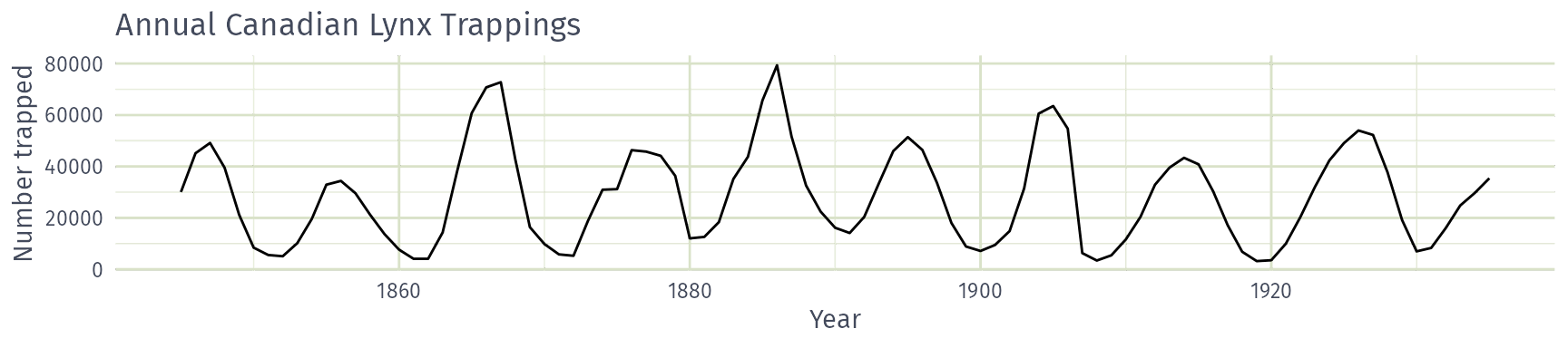
Annual Canadian lynx trappings: seasonal, cyclic, both or neither?

• Seasonal
• Cyclic
• Both
• Neither

Seasonal or cyclic?

Differences between seasonal and cyclic patterns:

• seasonal pattern constant length; cyclic pattern variable length
• average length of cycle longer than length of seasonal pattern
• magnitude of cycle more variable than magnitude of seasonal pattern

The timing of peaks and troughs is predictable with seasonal data, but unpredictable in the long term with cyclic data.

Lag plots and autocorrelation

Example: Beer production

new_production <- aus_production |>
  filter(year(Quarter) >= 1992)
new_production

# A tsibble: 74 x 7 [1Q]
   Quarter  Beer Tobacco Bricks Cement Electricity   Gas
     <qtr> <dbl>   <dbl>  <dbl>  <dbl>       <dbl> <dbl>
 1 1992 Q1   443    5777    383   1289       38332   117
 2 1992 Q2   410    5853    404   1501       39774   151
 3 1992 Q3   420    6416    446   1539       42246   175
 4 1992 Q4   532    5825    420   1568       38498   129
 5 1993 Q1   433    5724    394   1450       39460   116
 6 1993 Q2   421    6036    462   1668       41356   149
 7 1993 Q3   410    6570    475   1648       42949   163
 8 1993 Q4   512    5675    443   1863       40974   138
 9 1994 Q1   449    5311    421   1468       40162   127
10 1994 Q2   381    5717    475   1755       41199   159
# ℹ 64 more rows

Example: Beer production

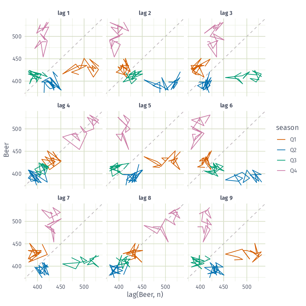
new_production |> gg_lag(Beer)

Example: Beer production

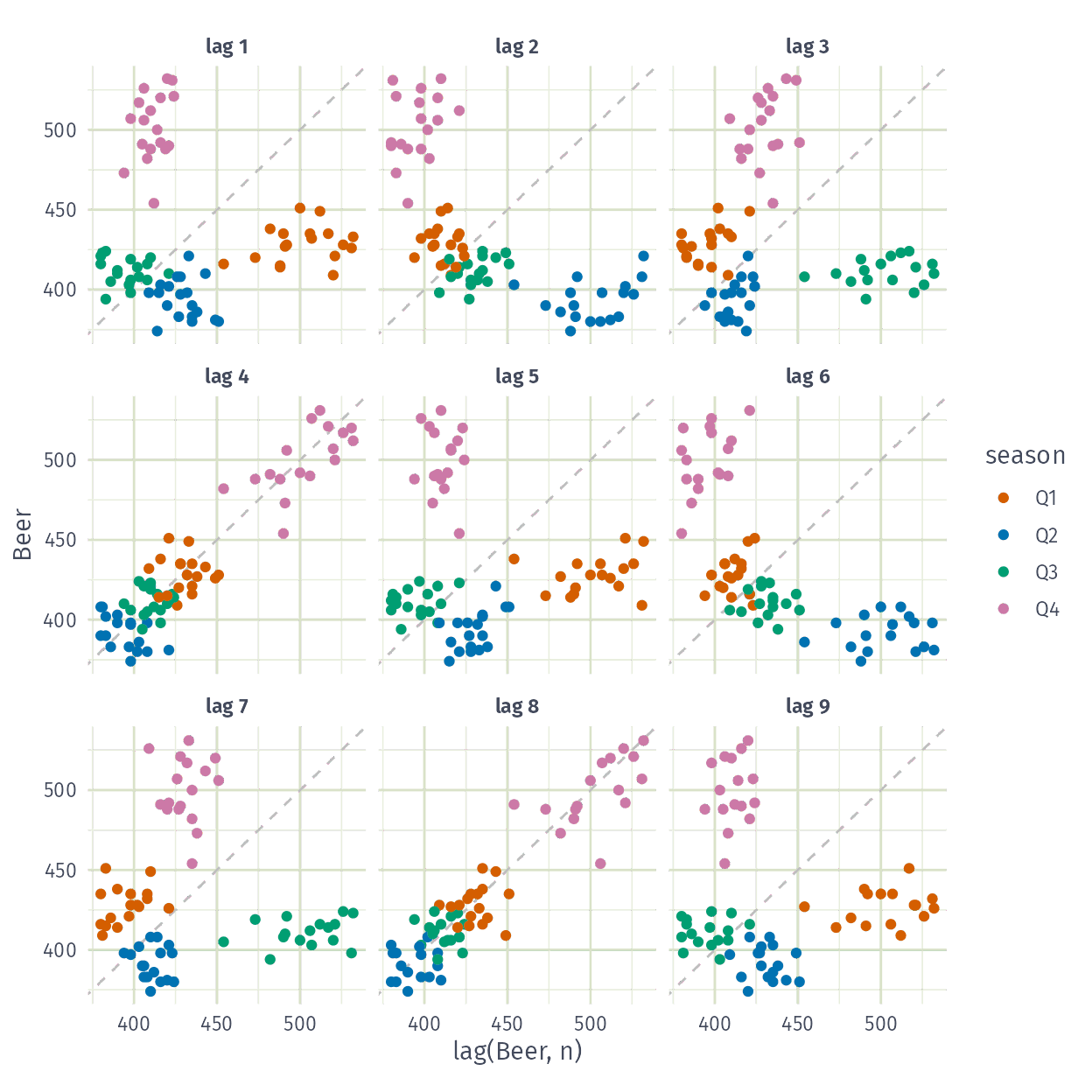
new_production |> gg_lag(Beer, geom = "point")

Lagged scatterplots

• Each graph shows \(y_t\) plotted against \(y_{t-k}\) for different values of \(k\).
• The autocorrelations are the correlations associated with these scatterplots.
• ACF (autocorrelation function):
  • \(r_1=\text{Correlation}(y_{t}, y_{t-1})\)
  • \(r_2=\text{Correlation}(y_{t}, y_{t-2})\)
  • \(r_3=\text{Correlation}(y_{t}, y_{t-3})\)
  • etc.
• If there is seasonality, the ACF at the seasonal lag (e.g., 12 for monthly data) will be large and positive.

From lag plots to the ACF

Time plot of quarterly Australian beer production since 1992.

Shift a copy of the series (orange) by one quarter, pairing each observation with the one before it.

Each pair is a point in the lag plot: \(y_t\) against \(y_{t-1}\). The first observation has no pair, so it is dropped.

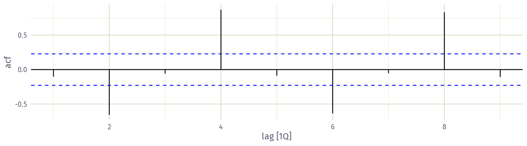
The autocorrelation \(r_1\) measures the linear relationship in this lag plot (orange line). It is small and negative: the first ACF bar.

Shift the copy by another quarter. At lag 2, each quarter is paired with the quarter half a year earlier, so the seasonality is out of phase: peaks are paired with troughs, and \(r_2\) is strongly negative.

Shift the copy by another quarter. At lag 3, each quarter is paired with the following quarter of the previous year. Like lag 1, these are neighbouring quarters, so \(r_3\) is close to zero.

Shift the copy to lag 4. Now each quarter is paired with the same quarter a year earlier, so the seasonal peaks and troughs line up: \(r_4\) is large and positive.

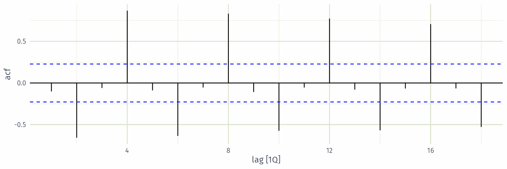
Continue for lags 5, 6, … The seasonal lags 8, 12 and 16 also align the same quarters, so they are strongly positive too.

The ACF plot. Dashed blue lines indicate 95% significance thresholds to help identify white noise.

Autocorrelation

Results for first 9 lags for beer data:

new_production |> ACF(Beer, lag_max = 9)

# A tsibble: 9 x 2 [1Q]
        lag     acf
   <cf_lag>   <dbl>
1 1 quarter -0.102 
2 2 quarter -0.657 
3 3 quarter -0.0603
4 4 quarter  0.869 
5 5 quarter -0.0892
6 6 quarter -0.635 
7 7 quarter -0.0542
8 8 quarter  0.832 
9 9 quarter -0.108 

Autocorrelation

Results for first 9 lags for beer data:

new_production |>
  ACF(Beer, lag_max = 9) |>
  autoplot()

ACF

new_production |>
  ACF(Beer) |>
  autoplot()

Australian holidays

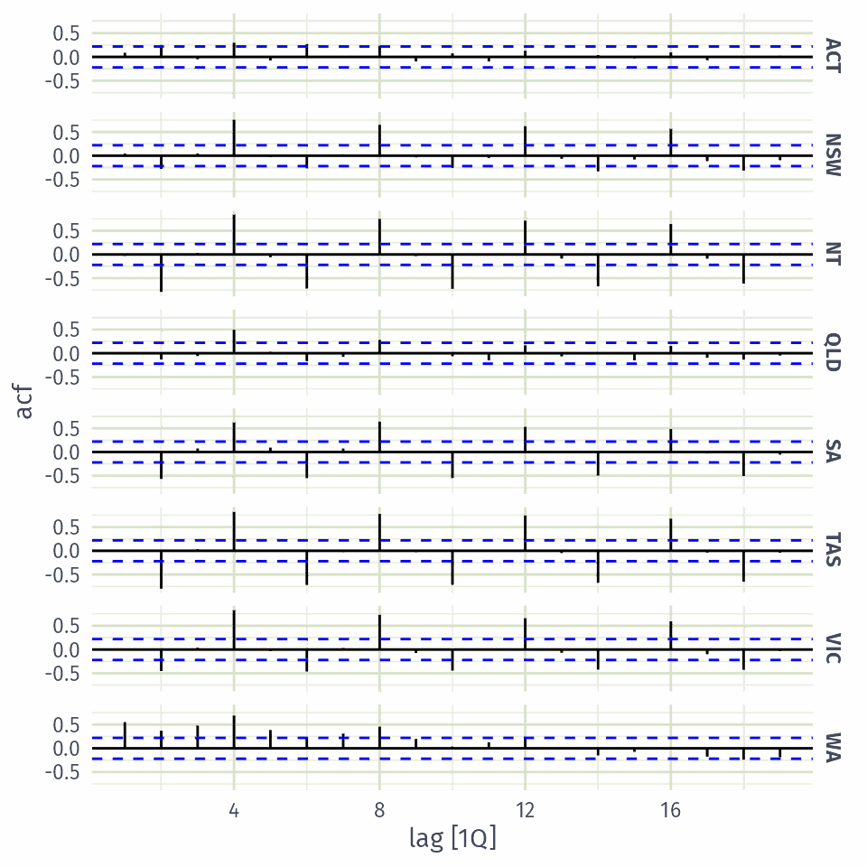
holidays |> ACF(Trips)

# A tsibble: 152 x 3 [1Q]
# Key:       State [8]
   State        lag      acf
   <chr>   <cf_lag>    <dbl>
 1 ACT    1 quarter  0.0877 
 2 ACT    2 quarter  0.252  
 3 ACT    3 quarter -0.0496 
 4 ACT    4 quarter  0.300  
 5 ACT    5 quarter -0.0741 
 6 ACT    6 quarter  0.269  
 7 ACT    7 quarter -0.00504
 8 ACT    8 quarter  0.236  
 9 ACT    9 quarter -0.0953 
10 ACT   10 quarter  0.0750 
# ℹ 142 more rows

Australian holidays

holidays |> ACF(Trips) |> autoplot()

Trend and seasonality in ACF plots

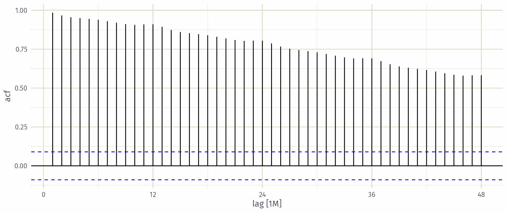
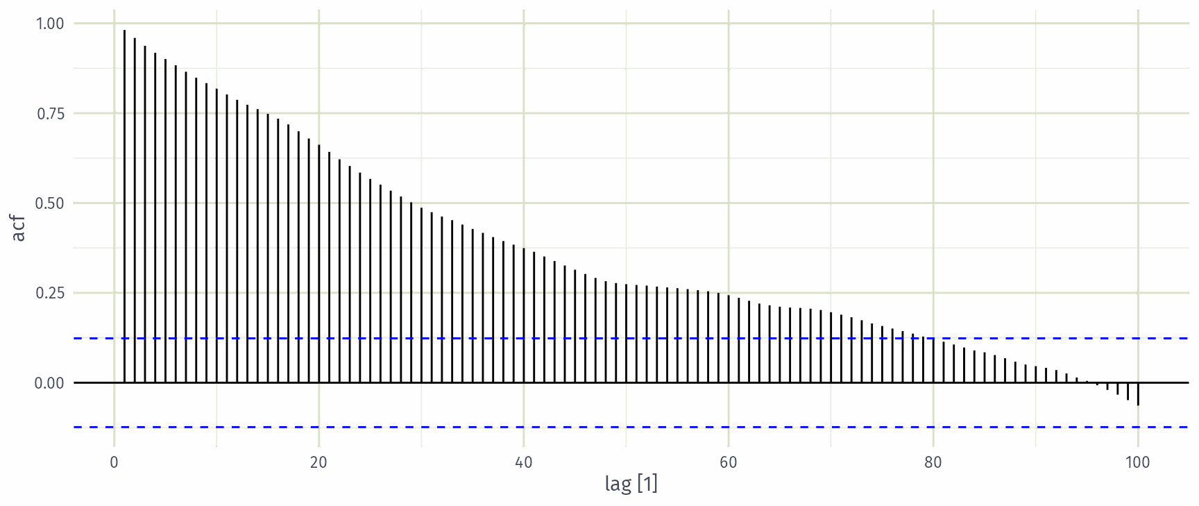
• When data have a trend, the autocorrelations for small lags tend to be large and positive.
• When data are seasonal, the autocorrelations will be larger at the seasonal lags (i.e., at multiples of the seasonal frequency)
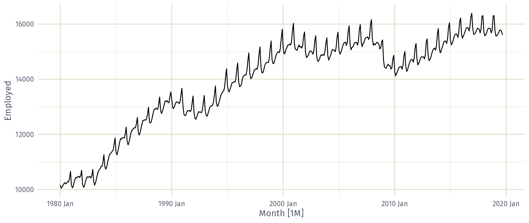
• When data are trended and seasonal, you see a combination of these effects.

US retail trade employment

retail <- us_employment |>
  filter(Title == "Retail Trade", year(Month) >= 1980)
retail |> autoplot(Employed)

US retail trade employment

retail |>
  ACF(Employed, lag_max = 48) |>
  autoplot()

Google stock price

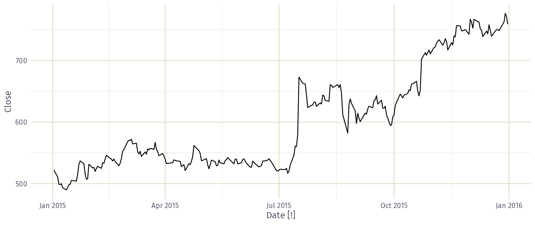
google_2015 <- gafa_stock |>
  filter(Symbol == "GOOG", year(Date) == 2015) |>
  select(Date, Close)
google_2015

# A tsibble: 252 x 2 [!]
   Date       Close
   <date>     <dbl>
 1 2015-01-02  522.
 2 2015-01-05  511.
 3 2015-01-06  499.
 4 2015-01-07  498.
 5 2015-01-08  500.
 6 2015-01-09  493.
 7 2015-01-12  490.
 8 2015-01-13  493.
 9 2015-01-14  498.
10 2015-01-15  499.
# ℹ 242 more rows

Google stock price

google_2015 |> autoplot(Close)

Google stock price

google_2015 |>
  ACF(Close, lag_max = 100) |>
  autoplot()

Which is which?

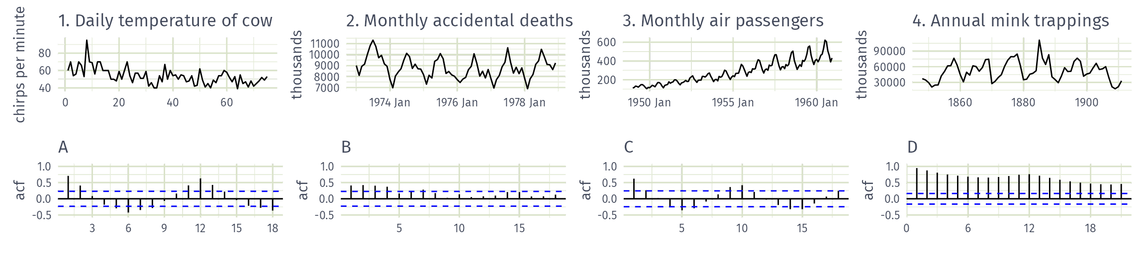
Match each time series (1-4) to its ACF (A-D)

• 1A, 2B, 3C, 4D
• 1B, 2A, 3D, 4C
• 1B, 2D, 3A, 4C
• 1C, 2A, 3D, 4B

White noise

Example: White noise

set.seed(4)
wn <- tsibble(t = seq(36), y = rnorm(36), index = t)
wn |> autoplot(y)

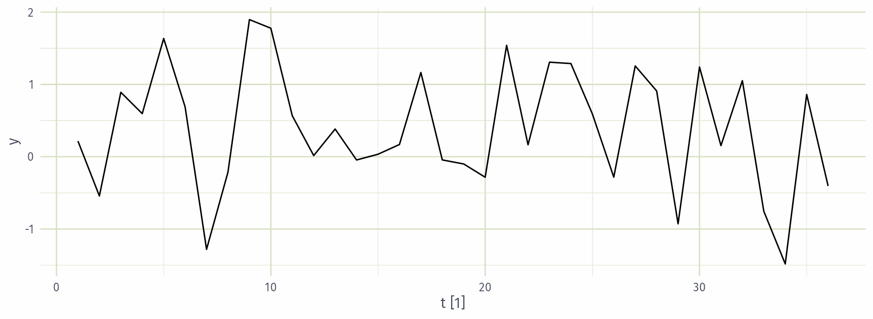
White noise data is uncorrelated across time with zero mean and constant variance.

(Technically, we require independence as well.)

Example: White noise

wn |> ACF(y)

\(r_{1}\)	\(r_{2}\)	\(r_{3}\)	\(r_{4}\)	\(r_{5}\)	\(r_{6}\)	\(r_{7}\)	\(r_{8}\)	\(r_{9}\)	\(r_{10}\)
0.001	-0.216	-0.144	0.033	0.126	-0.039	0.100	-0.051	-0.198	-0.198

• Sample autocorrelations for white noise series.
• Expect each autocorrelation to be close to zero.
• Blue lines show 95% critical values.

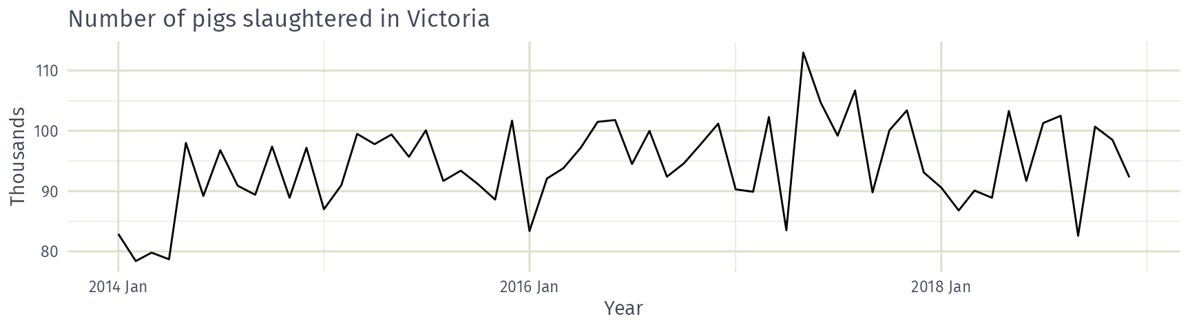
Example: Pigs slaughtered

pigs <- aus_livestock |>
  filter(State == "Victoria", Animal == "Pigs", year(Month) >= 2014)
pigs |> autoplot(Count / 1e3) +
  labs(x = "Year", y = "Thousands",
       title = "Number of pigs slaughtered in Victoria")

Example: Pigs slaughtered

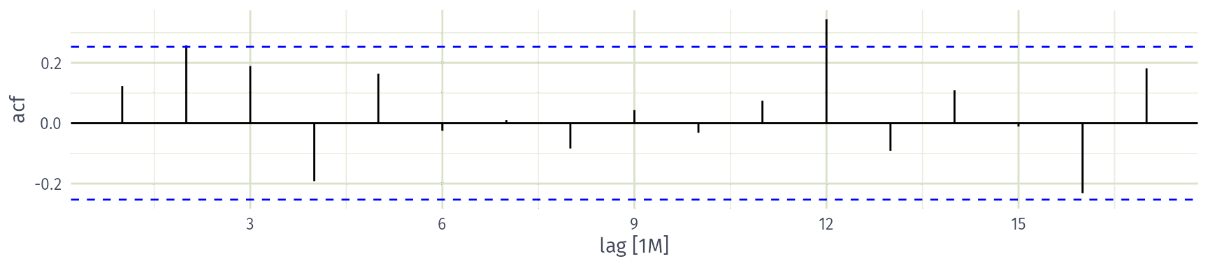
Is the number of pigs slaughtered a white noise series?

• Yes
• No

Example: Pigs slaughtered

Monthly total number of pigs slaughtered in the state of Victoria, Australia, from January 2014 through December 2018 (Source: Australian Bureau of Statistics.)

• Difficult to detect pattern in time plot.
• ACF shows significant autocorrelation for lag 2 and 12.
• Indicate some slight seasonality.

These show the series is not a white noise series.