AFRICAST

Tidy time series & forecasting in R

Basics of time series and data structures

Session 1 of 10

workshop.f4sg.org/africastForecasting for Social Good

Introduction to forecasting

What is a forecast?

Estimating how a sequence of observations will continue into the future, using all information available now.

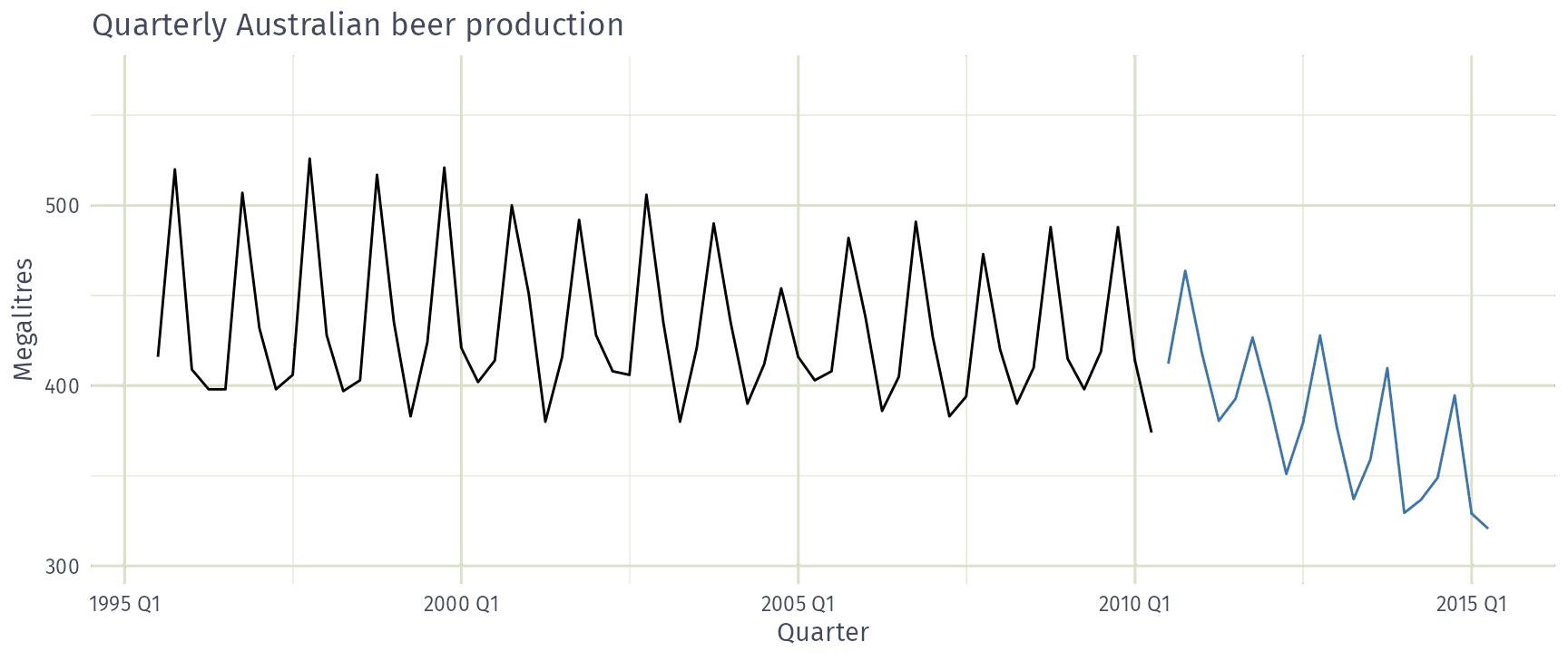
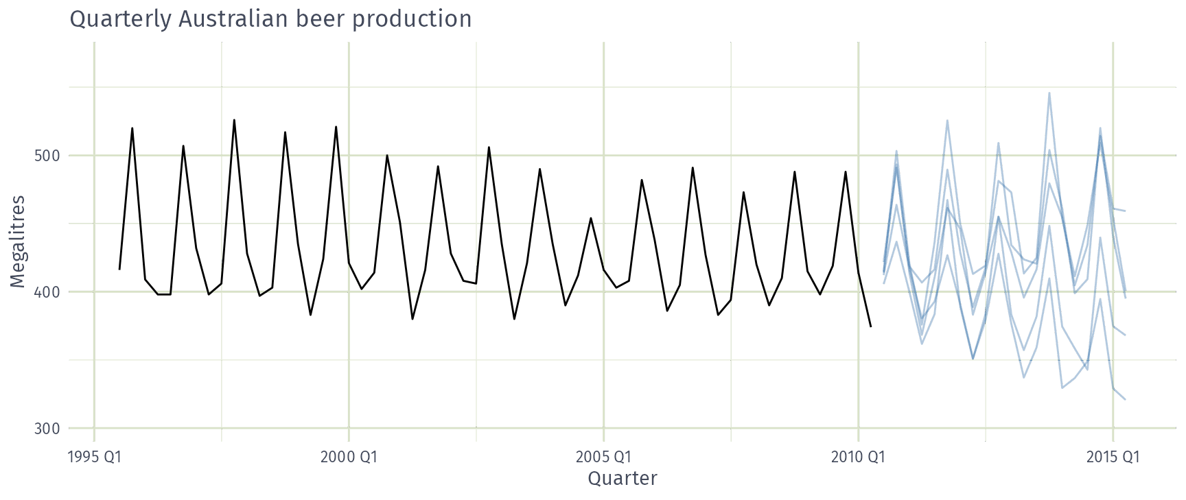
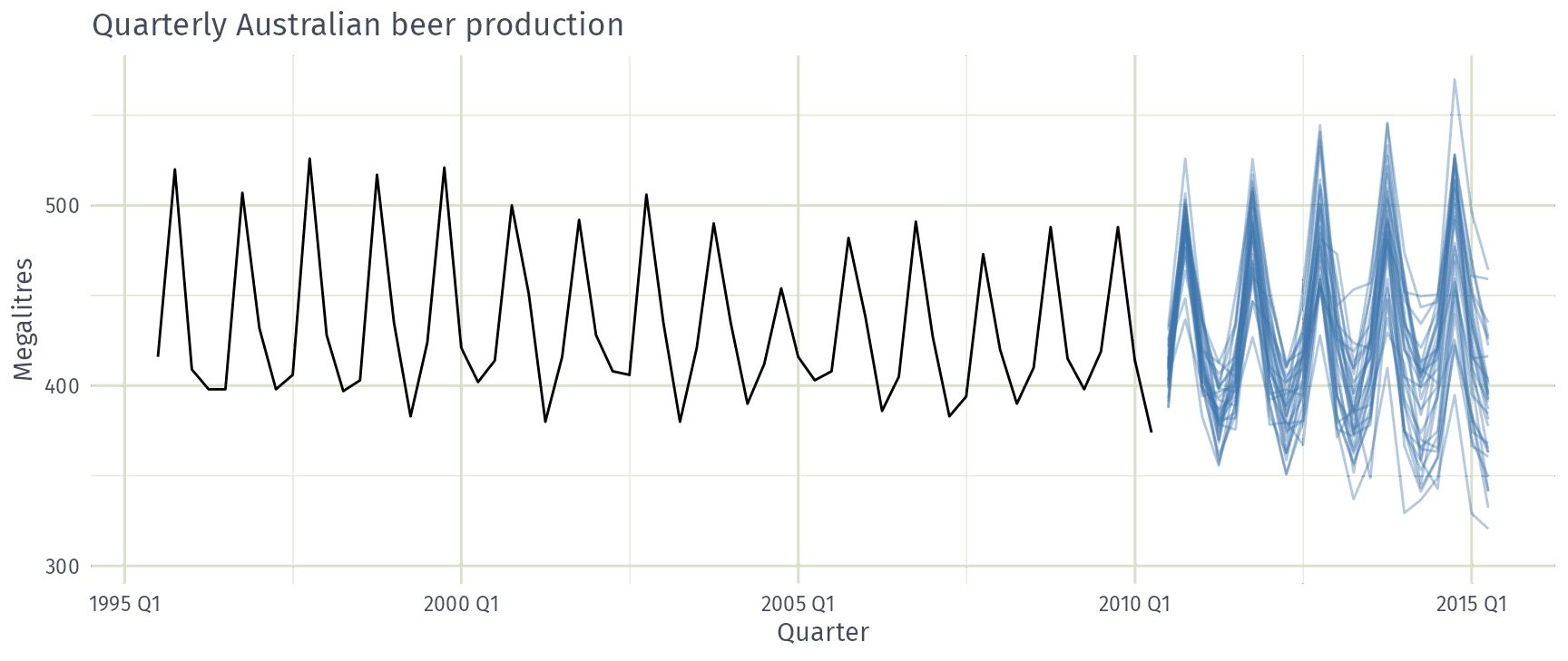
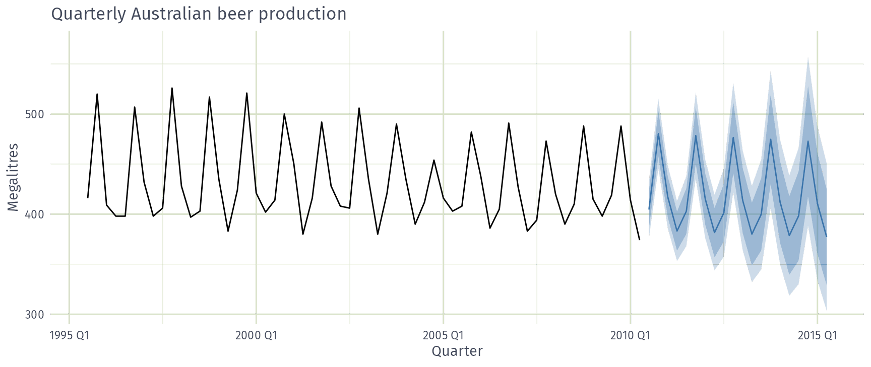
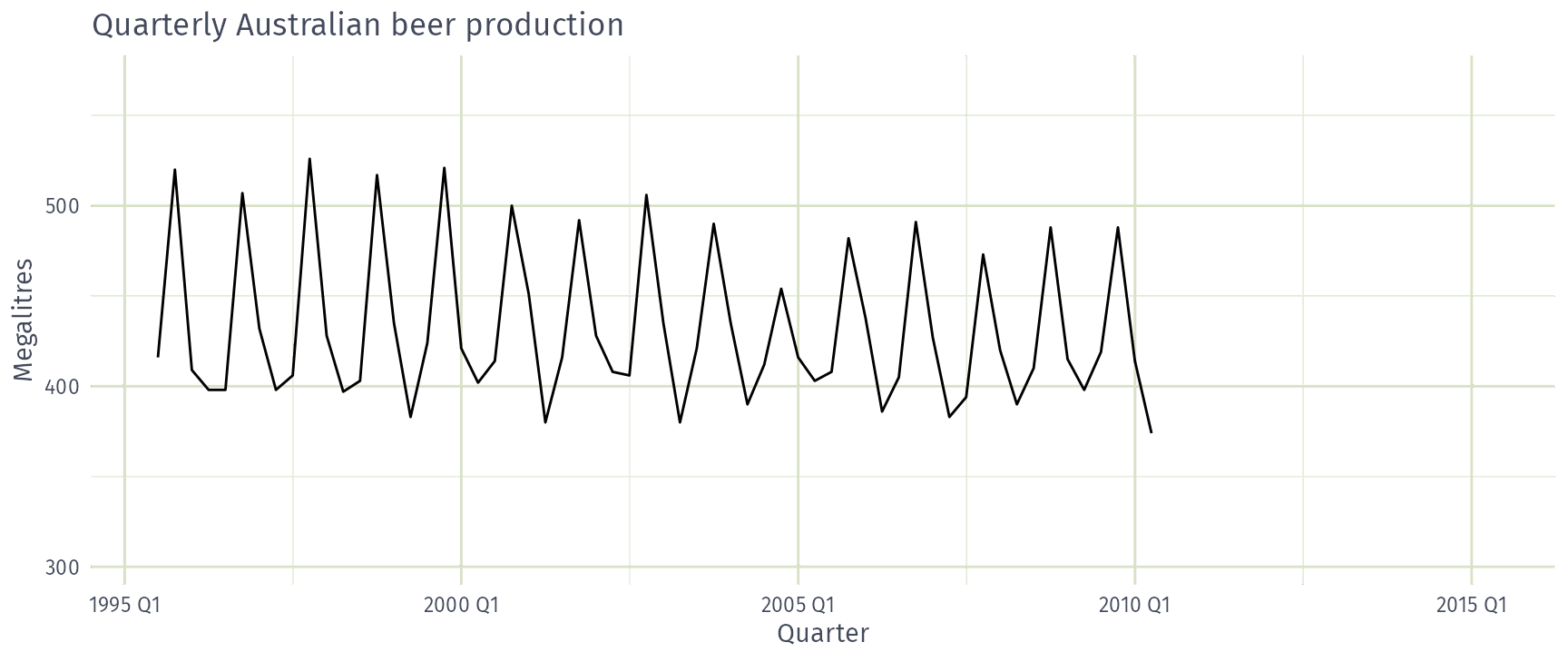
What data do we need?

Historical data on the variable to forecast
Past and future values of predictors
- Deterministic (e.g. holidays)
- Stochastic (e.g. temperature)
Expert knowledge and context
- New information

Why forecast?

Why do you use forecasts?

Decision	Forecast
Build a new hospital in the next 10 years?	Population and patient demand, years ahead
Call centre staff needed next week?	Call volumes, hours to days ahead
Vaccine doses needed next month?	Doses by region, weeks ahead

The decision sets what to forecast and how far ahead.

Forecasting workflow

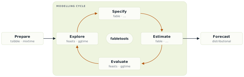
Packages for this course

tidyverts.org

Time series data

Example datasets

Features and decompositions

Time series graphics

Forecasting models

Packages for this course

# Data, graphics and forecasting
library(fpp3)

-- Attaching packages ------------------------------ fpp3 1.0.3 --

v tibble      3.3.1          v tsibble     1.2.0.9000
v dplyr       1.2.1          v tsibbledata 0.4.1     
v tidyr       1.3.2          v ggtime      1.1.0.9000
v lubridate   1.9.5          v feasts      0.5.0.9000
v ggplot2     4.0.3          v fable       0.5.0.9000

Time series data

Four-yearly Olympic winning times
Annual Google profits
Quarterly Australian beer production
Monthly rainfall
Weekly retail sales
Daily IBM stock prices
Hourly electricity demand
5-minute freeway traffic counts
Time-stamped stock transaction data

Your time series

What time series data do you work with?

What makes it a time series?

Observations + when they happened.

The time column is the index
Observations are ordered in time
Regular intervals define the frequency (yearly, quarterly, …)

tsibble objects

A `tsibble` has three parts

A tsibble stores one or more time series in a table.

Index: when
Key: which series (optional)
Measures: what was observed

Works with dplyr verbs (filter(), mutate(), …).

`tsibble` objects

global_economy

# A tsibble: 15,150 x 6 [1Y]
# Key:       Country [263]
    Year Country             GDP Imports Exports Population
   <dbl> <fct>             <dbl>   <dbl>   <dbl>      <dbl>
 1  1960 Afghanistan  537777811.    7.02    4.13    8996351
 2  1961 Afghanistan  548888896.    8.10    4.45    9166764
 3  1962 Afghanistan  546666678.    9.35    4.88    9345868
 4  1963 Afghanistan  751111191.   16.9     9.17    9533954
 5  1964 Afghanistan  800000044.   18.1     8.89    9731361
 6  1965 Afghanistan 1006666638.   21.4    11.3     9938414
 7  1966 Afghanistan 1399999967.   18.6     8.57   10152331
 8  1967 Afghanistan 1673333418.   14.2     6.77   10372630
 9  1968 Afghanistan 1373333367.   15.2     8.90   10604346
10  1969 Afghanistan 1408888922.   15.0    10.1    10854428
# ℹ 15,140 more rows

Index

Key

Measures

`tsibble` objects

tourism

# A tsibble: 24,320 x 5 [1Q]
# Key:       Region, State, Purpose [304]
   Quarter Region   State Purpose  Trips
     <qtr> <chr>    <chr> <chr>    <dbl>
 1 1998 Q1 Adelaide SA    Business  135.
 2 1998 Q2 Adelaide SA    Business  110.
 3 1998 Q3 Adelaide SA    Business  166.
 4 1998 Q4 Adelaide SA    Business  127.
 5 1999 Q1 Adelaide SA    Business  137.
 6 1999 Q2 Adelaide SA    Business  200.
 7 1999 Q3 Adelaide SA    Business  169.
 8 1999 Q4 Adelaide SA    Business  134.
 9 2000 Q1 Adelaide SA    Business  154.
10 2000 Q2 Adelaide SA    Business  169.
# ℹ 24,310 more rows

Index

Keys

Measure

Overnight trips (thousands), quarterly, by region and purpose of travel.

The `tsibble` index

For annual data, integer years work as the index:

annual_data <- tsibble(
  year = 2012:2016,
  y = c(123, 39, 78, 52, 110),
  index = year
)
annual_data

# A tsibble: 5 x 2 [1Y]
   year     y
  <int> <dbl>
1  2012   123
2  2013    39
3  2014    78
4  2015    52
5  2016   110

The `tsibble` index

monthly_data

# A tibble: 5 × 2
  Month    Observation
  <chr>          <dbl>
1 2019 Jan          50
2 2019 Feb          23
3 2019 Mar          34
4 2019 Apr          30
5 2019 May          25

"2019 Jan" is just text
More frequent than yearly? Use a time class

The `tsibble` index

monthly_data |>
  mutate(Month = yearmonth(Month)) |>
  as_tsibble(index = Month)

# A tsibble: 5 x 2 [1M]
     Month Observation
     <mth>       <dbl>
1 2019 Jan          50
2 2019 Feb          23
3 2019 Mar          34
4 2019 Apr          30
5 2019 May          25

The `tsibble` index

Common time index variables can be created with these functions:

Frequency	Function
Annual	`start:end`
Quarterly	`yearquarter()`
Monthly	`yearmonth()`
Weekly	`yearweek()`
Daily	`as_date()`, `ymd()`
Sub-daily	`as_datetime()`, `ymd_hms()`

Converting dates

Often data is provided as dates, even if it isn’t daily.

my_date <- as.Date("2026-10-01")
yearquarter(my_date)

<yearquarter[1]>
[1] "2026 Q4"
# Year starts on: January

yearmonth(my_date)

<yearmonth[1]>
[1] "2026 Oct"

yearweek(my_date)

<yearweek[1]>
[1] "2026 W40"
# Week starts on: Monday

Looking ahead: `mixtime`

One family of linear time classes, including year() and datetime():

library(mixtime)
c(year(my_date), yearquarter(my_date), yearmonth(my_date), date(my_date))

<mixtime[4]>
[1] 2026       2026 Q4    2026 Oct   2026-10-01

Any granularity: pick a chronon (one time step) and call linear_time():

quarter_hours <- datetime("2024-01-01 00:00:00") + minutes(0:3) * 15L
linear_time(quarter_hours, chronon = cal_gregorian$minute(15L))

<mixtime[4]>
[1] 2024-01-01 00:00 2024-01-01 00:15 2024-01-01 00:30 2024-01-01 00:45

yearmonth(my_date) is linear_time(my_date, chronon = cal_gregorian$month(1L))

Looking ahead: `mixtime`

More time types, beyond this course:

# Timezones
datetime(as.POSIXct("2026-10-05 22:30", tz = "UTC"), tz = "Africa/Nairobi")

<mixtime[1]>
[1] 2026-10-06 01:30:00 EAT

# Other calendars (also cal_isoweek, lunar and solar calendars)
linear_time(my_date, chronon = cal_sym454$month(1L))

<mixtime[1]>
[1] 2026-Oct

# Cyclical time
day_of_week(my_date)

<mixtime[1]>
[1] Thu

# Durations
yearmonth(my_date) + months(0:2)

<mixtime[3]>
[1] 2026 Oct 2026 Nov 2026 Dec

What a `tsibble` checks

Index + key must uniquely identify each row: as_tsibble() errors on duplicates (find them with duplicates())
The interval is shown in the header: [1Y], [1Q], [1M], …
Missing time steps are implicit gaps: find them with has_gaps(), make them explicit with fill_gaps()

tsibble(year = c(2012, 2013, 2015, 2016), y = c(123, 39, 52, 110), index = year) |>
  fill_gaps()

# A tsibble: 5 x 2 [1Y]
   year     y
  <dbl> <dbl>
1  2012   123
2  2013    39
3  2014    NA
4  2015    52
5  2016   110

Example: Australian prison population

Australian prison population

Read a csv file

Quarterly prisoner counts from the ABS, 2005 Q1 to 2016 Q4, by state, gender, legal status and indigenous status (ATSI: Aboriginal and Torres Strait Islander).

prison <- readr::read_csv("data/prison_population.csv")

# A tibble: 3,072 × 6
   date       state gender legal     indigenous count
   <date>     <chr> <chr>  <chr>     <chr>      <dbl>
 1 2005-03-01 ACT   Female Remanded  ATSI           0
 2 2005-03-01 ACT   Female Remanded  Other          2
 3 2005-03-01 ACT   Female Sentenced ATSI           0
 4 2005-03-01 ACT   Female Sentenced Other          0
 5 2005-03-01 ACT   Male   Remanded  ATSI           7
 6 2005-03-01 ACT   Male   Remanded  Other         58
 7 2005-03-01 ACT   Male   Sentenced ATSI           0
 8 2005-03-01 ACT   Male   Sentenced Other          0
 9 2005-03-01 NSW   Female Remanded  ATSI          51
10 2005-03-01 NSW   Female Remanded  Other        131
# ℹ 3,062 more rows

Convert to a time class

prison <- readr::read_csv("data/prison_population.csv") |>
  mutate(quarter = yearquarter(date))

# A tibble: 3,072 × 7
   date       state gender legal     indigenous count quarter
   <date>     <chr> <chr>  <chr>     <chr>      <dbl>   <qtr>
 1 2005-03-01 ACT   Female Remanded  ATSI           0 2005 Q1
 2 2005-03-01 ACT   Female Remanded  Other          2 2005 Q1
 3 2005-03-01 ACT   Female Sentenced ATSI           0 2005 Q1
 4 2005-03-01 ACT   Female Sentenced Other          0 2005 Q1
 5 2005-03-01 ACT   Male   Remanded  ATSI           7 2005 Q1
 6 2005-03-01 ACT   Male   Remanded  Other         58 2005 Q1
 7 2005-03-01 ACT   Male   Sentenced ATSI           0 2005 Q1
 8 2005-03-01 ACT   Male   Sentenced Other          0 2005 Q1
 9 2005-03-01 NSW   Female Remanded  ATSI          51 2005 Q1
10 2005-03-01 NSW   Female Remanded  Other        131 2005 Q1
# ℹ 3,062 more rows

Remove the old date column

prison <- readr::read_csv("data/prison_population.csv") |>
  mutate(quarter = yearquarter(date)) |>
  select(-date)

# A tibble: 3,072 × 6
   state gender legal     indigenous count quarter
   <chr> <chr>  <chr>     <chr>      <dbl>   <qtr>
 1 ACT   Female Remanded  ATSI           0 2005 Q1
 2 ACT   Female Remanded  Other          2 2005 Q1
 3 ACT   Female Sentenced ATSI           0 2005 Q1
 4 ACT   Female Sentenced Other          0 2005 Q1
 5 ACT   Male   Remanded  ATSI           7 2005 Q1
 6 ACT   Male   Remanded  Other         58 2005 Q1
 7 ACT   Male   Sentenced ATSI           0 2005 Q1
 8 ACT   Male   Sentenced Other          0 2005 Q1
 9 NSW   Female Remanded  ATSI          51 2005 Q1
10 NSW   Female Remanded  Other        131 2005 Q1
# ℹ 3,062 more rows

Declare the index and keys

prison <- readr::read_csv("data/prison_population.csv") |>
  mutate(quarter = yearquarter(date)) |>
  select(-date) |>
  as_tsibble(
    index = quarter,
    key = c(state, gender, legal, indigenous)
  )

# A tsibble: 3,072 x 6 [1Q]
# Key:       state, gender, legal, indigenous [64]
   state gender legal    indigenous count quarter
   <chr> <chr>  <chr>    <chr>      <dbl>   <qtr>
 1 ACT   Female Remanded ATSI           0 2005 Q1
 2 ACT   Female Remanded ATSI           1 2005 Q2
 3 ACT   Female Remanded ATSI           0 2005 Q3
 4 ACT   Female Remanded ATSI           0 2005 Q4
 5 ACT   Female Remanded ATSI           1 2006 Q1
 6 ACT   Female Remanded ATSI           1 2006 Q2
 7 ACT   Female Remanded ATSI           1 2006 Q3
 8 ACT   Female Remanded ATSI           0 2006 Q4
 9 ACT   Female Remanded ATSI           0 2007 Q1
10 ACT   Female Remanded ATSI           1 2007 Q2
# ℹ 3,062 more rows

Example: Australian pharmaceutical sales

Australian Pharmaceutical Benefits Scheme

The PBS is the Australian government drug subsidy scheme.

Subsidises many pharmacy drugs
Cost the government A$19.1 billion in 2024–25 (about 0.7% of GDP)
Budget relies on forecasts of drug usage

PBS data: monthly, July 1991 to June 2008

Scripts (prescriptions) and Cost (A$)
By drug type (ATC2 x84), concession (x2) and patient type (x2)
ATC: Anatomical Therapeutic Chemical classification

Working with `tsibble` objects

PBS

# A tsibble: 67,596 x 9 [1M]
# Key:       Concession, Type, ATC1, ATC2 [336]
      Month Concession   Type        ATC1  ATC1_desc                   ATC2  ATC2_desc Scripts  Cost
      <mth> <chr>        <chr>       <chr> <chr>                       <chr> <chr>       <dbl> <dbl>
 1 1991 Jul Concessional Co-payments A     Alimentary tract and metab… A01   STOMATOL…   18228 67877
 2 1991 Aug Concessional Co-payments A     Alimentary tract and metab… A01   STOMATOL…   15327 57011
 3 1991 Sep Concessional Co-payments A     Alimentary tract and metab… A01   STOMATOL…   14775 55020
 4 1991 Oct Concessional Co-payments A     Alimentary tract and metab… A01   STOMATOL…   15380 57222
 5 1991 Nov Concessional Co-payments A     Alimentary tract and metab… A01   STOMATOL…   14371 52120
 6 1991 Dec Concessional Co-payments A     Alimentary tract and metab… A01   STOMATOL…   15028 54299
 7 1992 Jan Concessional Co-payments A     Alimentary tract and metab… A01   STOMATOL…   11040 39753
 8 1992 Feb Concessional Co-payments A     Alimentary tract and metab… A01   STOMATOL…   15165 54405
 9 1992 Mar Concessional Co-payments A     Alimentary tract and metab… A01   STOMATOL…   16898 61108
10 1992 Apr Concessional Co-payments A     Alimentary tract and metab… A01   STOMATOL…   18141 65356
# ℹ 67,586 more rows

`filter()`: choose rows

PBS |>
  filter(ATC2 == "A10")

# A tsibble: 816 x 9 [1M]
# Key:       Concession, Type, ATC1, ATC2 [4]
      Month Concession   Type        ATC1  ATC1_desc                  ATC2  ATC2_desc Scripts   Cost
      <mth> <chr>        <chr>       <chr> <chr>                      <chr> <chr>       <dbl>  <dbl>
 1 1991 Jul Concessional Co-payments A     Alimentary tract and meta… A10   ANTIDIAB…   89733 2.09e6
 2 1991 Aug Concessional Co-payments A     Alimentary tract and meta… A10   ANTIDIAB…   77101 1.80e6
 3 1991 Sep Concessional Co-payments A     Alimentary tract and meta… A10   ANTIDIAB…   76255 1.78e6
 4 1991 Oct Concessional Co-payments A     Alimentary tract and meta… A10   ANTIDIAB…   78681 1.85e6
 5 1991 Nov Concessional Co-payments A     Alimentary tract and meta… A10   ANTIDIAB…   70554 1.69e6
 6 1991 Dec Concessional Co-payments A     Alimentary tract and meta… A10   ANTIDIAB…   75814 1.84e6
 7 1992 Jan Concessional Co-payments A     Alimentary tract and meta… A10   ANTIDIAB…   64186 1.56e6
 8 1992 Feb Concessional Co-payments A     Alimentary tract and meta… A10   ANTIDIAB…   75899 1.73e6
 9 1992 Mar Concessional Co-payments A     Alimentary tract and meta… A10   ANTIDIAB…   89445 2.05e6
10 1992 Apr Concessional Co-payments A     Alimentary tract and meta… A10   ANTIDIAB…   97315 2.23e6
# ℹ 806 more rows

`select()`: choose columns

PBS |>
  filter(ATC2 == "A10") |>
  select(Month, Concession, Type, Cost)

# A tsibble: 816 x 4 [1M]
# Key:       Concession, Type [4]
      Month Concession   Type           Cost
      <mth> <chr>        <chr>         <dbl>
 1 1991 Jul Concessional Co-payments 2092878
 2 1991 Aug Concessional Co-payments 1795733
 3 1991 Sep Concessional Co-payments 1777231
 4 1991 Oct Concessional Co-payments 1848507
 5 1991 Nov Concessional Co-payments 1686458
 6 1991 Dec Concessional Co-payments 1843079
 7 1992 Jan Concessional Co-payments 1564702
 8 1992 Feb Concessional Co-payments 1732508
 9 1992 Mar Concessional Co-payments 2046102
10 1992 Apr Concessional Co-payments 2225977
# ℹ 806 more rows

`summarise()`: combine over keys

PBS |>
  filter(ATC2 == "A10") |>
  select(Month, Concession, Type, Cost) |>
  summarise(total_cost = sum(Cost))

# A tsibble: 204 x 2 [1M]
      Month total_cost
      <mth>      <dbl>
 1 1991 Jul    3526591
 2 1991 Aug    3180891
 3 1991 Sep    3252221
 4 1991 Oct    3611003
 5 1991 Nov    3565869
 6 1991 Dec    4306371
 7 1992 Jan    5088335
 8 1992 Feb    2814520
 9 1992 Mar    2985811
10 1992 Apr    3204780
# ℹ 194 more rows

`mutate()`: create variables

PBS |>
  filter(ATC2 == "A10") |>
  select(Month, Concession, Type, Cost) |>
  summarise(total_cost = sum(Cost)) |>
  mutate(cost_m = total_cost / 1e6)

# A tsibble: 204 x 3 [1M]
      Month total_cost cost_m
      <mth>      <dbl>  <dbl>
 1 1991 Jul    3526591   3.53
 2 1991 Aug    3180891   3.18
 3 1991 Sep    3252221   3.25
 4 1991 Oct    3611003   3.61
 5 1991 Nov    3565869   3.57
 6 1991 Dec    4306371   4.31
 7 1992 Jan    5088335   5.09
 8 1992 Feb    2814520   2.81
 9 1992 Mar    2985811   2.99
10 1992 Apr    3204780   3.20
# ℹ 194 more rows

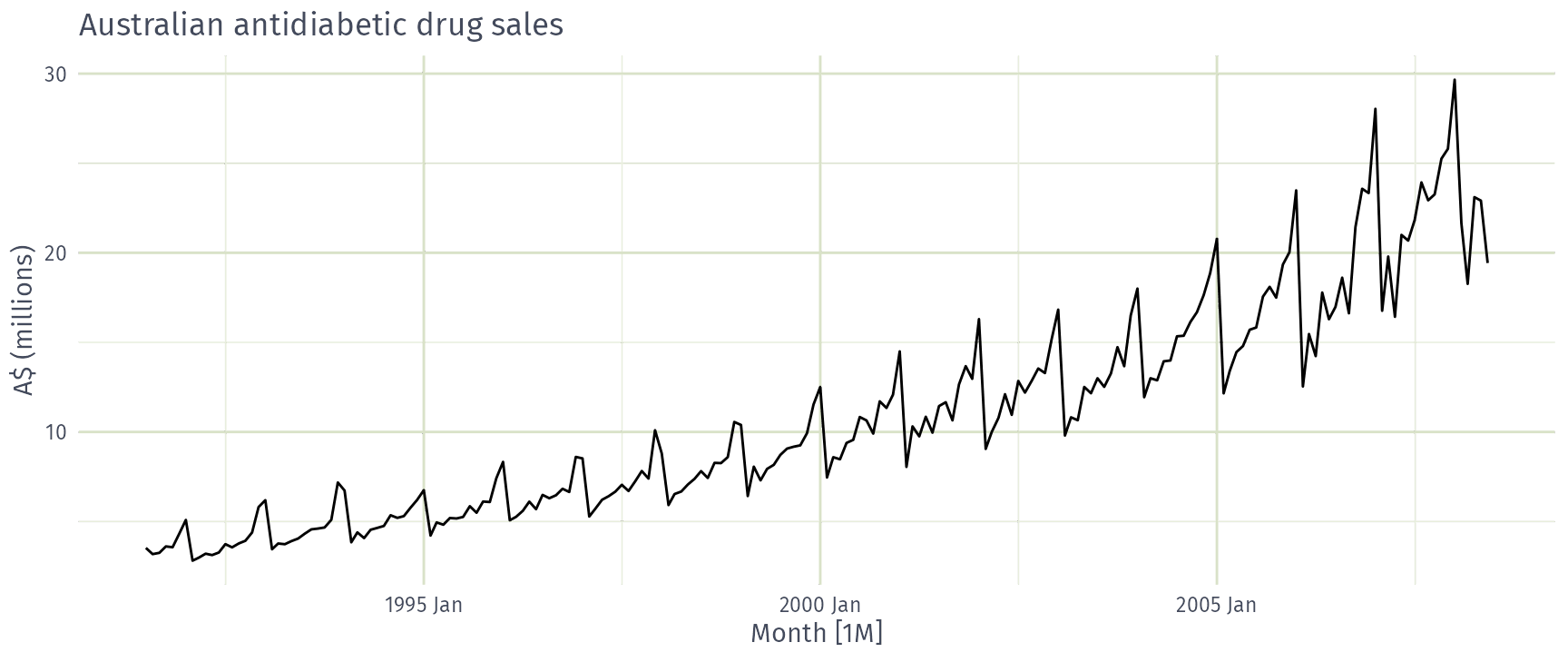
cost_m is the total cost in A$ millions.

Save the result

a10 <- PBS |>
  filter(ATC2 == "A10") |>
  select(Month, Concession, Type, Cost) |>
  summarise(total_cost = sum(Cost)) |>
  mutate(cost_m = total_cost / 1e6)

# A tsibble: 204 x 3 [1M]
      Month total_cost cost_m
      <mth>      <dbl>  <dbl>
 1 1991 Jul    3526591   3.53
 2 1991 Aug    3180891   3.18
 3 1991 Sep    3252221   3.25
 4 1991 Oct    3611003   3.61
 5 1991 Nov    3565869   3.57
 6 1991 Dec    4306371   4.31
 7 1992 Jan    5088335   5.09
 8 1992 Feb    2814520   2.81
 9 1992 Mar    2985811   2.99
10 1992 Apr    3204780   3.20
# ℹ 194 more rows

Plot the result

autoplot(a10, cost_m) +
  labs(y = "A$ (millions)", title = "Australian antidiabetic drug sales")

Your turn

Using tourism

Find the quarterly total Trips for each State
Challenge: Which State had the most Trips over the whole period?

Using PBS

Find the total monthly Scripts for ATC2 "H02"

Hints

summarise() always keeps the index
Q1: group_by(State), then summarise()
Q2: as_tibble() first: it drops the tsibble structure, so summarise() no longer keeps the index
Q3: filter(), then summarise()

Recap

A tsibble has an index, keys and measures
Index + keys uniquely identify each row
The index needs a time class (yearmonth(), as_date(), …)
Use dplyr verbs to wrangle tsibbles
summarise() combines over keys, keeping the index

Basics of time series and data structures

Introduction to forecasting

What is a forecast?

What data do we need?

Why forecast?

Forecasting workflow

Packages for this course

Packages for this course

Time series data

Time series data

Your time series

What makes it a time series?

tsibble objects

A tsibble has three parts

tsibble objects

tsibble objects

The tsibble index

The tsibble index

The tsibble index

The tsibble index

Converting dates

Looking ahead: mixtime

Looking ahead: mixtime

What a tsibble checks

Example: Australian prison population

Australian prison population

Read a csv file

Convert to a time class

Remove the old date column

Declare the index and keys

Example: Australian pharmaceutical sales

Australian Pharmaceutical Benefits Scheme

Australian Pharmaceutical Benefits Scheme

Working with tsibble objects

filter(): choose rows

select(): choose columns

summarise(): combine over keys

mutate(): create variables

Save the result

Plot the result

Your turn

Recap

A `tsibble` has three parts

`tsibble` objects

`tsibble` objects

The `tsibble` index

The `tsibble` index

The `tsibble` index

The `tsibble` index

Looking ahead: `mixtime`

Looking ahead: `mixtime`

What a `tsibble` checks

Working with `tsibble` objects

`filter()`: choose rows

`select()`: choose columns

`summarise()`: combine over keys

`mutate()`: create variables